Predefined Filters
Macro filter models are based at the lowest level on predefined filters that actually do computations to generate new statistic data. The top level macro filter and intermediate levels of macro filters merely serve to structure the user’s approach to designing a filter model that performs a particular computation.
The predefined filters can do a variety of computations including arithmetic, basic calculus, and statistical operations. Currently, there is no open interface for defining new filter models other than macro filters; as a result, fundamentally new types of computations cannot be performed with the filter facility. In the following sections, the terms unary and binary are used to refer to filters that require one and two inputs, respectively. Also, a filter can be assumed to have no parameters, unless these parameters are explicitly mentioned.
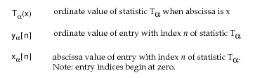
The descriptions of some of the filters include equations and tables to explain the computations that are performed. These tables and equations make use of the following notations:
Arithmetic Filters
Adder Filter
The “adder” filter is a binary filter used to combine two input statistics T₀ and T₁ to generate a third statistic, Tout, which represents their sum.
Table 138: Synopsis of Adder Filter
| Input Statistics | Parameters | Output |
|---|---|---|
| two interchangeable inputs | none | sum of two input statistics |
If the two input statistics T₀ and T₁ have exactly the same number of entries and these entries are aligned with respect to their abscissa values, then T_out can be computed simply by adding ordinate values for entries of equal abscissa, as follows:

However, if the input statistics are not initially perfectly aligned with respect to each other, then an abscissa alignment mechanism is automatically applied by this filter before adding is performed. Alignment consists of two steps:
- T₀ and T₁ are truncated to the same minimum and maximum abscissa values, by removing entries as necessary. This essentially corresponds to finding the intersection of the two statistics on the horizontal axis.
- The truncated statistics resulting from step 1 are augmented to ensure that each statistic contains entries at the same abscissas as the other; this involves inserting points into each of the statistics. For example, if the two statistics had no abscissa values in common, once augmented they would contain a number of entries equal to the sum of their original lengths. When an entry is inserted, its ordinate value is taken to be the ordinate value of the previous entry in the same statistic (i.e., it is assumed that the statistic’s ordinate value remains constant until the next original entry).
After alignment has completed, the two resulting statistics can be added directly, entry by entry. When adding entries, the rules presented in the following table are applied (because T₀ and T₁ are treated identically, the table’s corresponding column headings can be inverted to address symmetric cases).
Table 139: Entry Calculation Rules for Adder Filter
| T₀ | T₁ | T_out |
|---|---|---|
| a¹ | b | a + b |
| a | +infinity | +infinity |
| a | -infinity | -infinity |
| * | undefined | undefined |
| +infinity | +infinity | +infinity |
| -infinity | -infinity | -infinity |
| +infinity | -infinity | undefined |
Note 1: (a, b = real constants, * = any value)
Constant Shift Filter
The “constant_shift” filter is a unary filter used to operate on one input statistic T₀ to generate a second statistic, T_out, which is a translation of T₀ by an amount  along the direction of the vertical axis. The shift quantity
 is a real number specified as a parameter of the filter.
Table 140: Synopsis of Constant Shift Filter
| Input Statistics | Parameters | Output |
|---|---|---|
| single input | shift: translation distance along vertical axis | translated version of input statistic |
The T_out statistic has the same number of entries as T₀ and the two statistics are aligned with each other with respect to the entries’ abscissa values. Only the ordinate values differ by the constant  as follows:
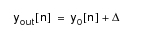
When computing the entries of T_out, the rules summarized in the following table are applied (the content of the T₀ and  columns can be interchanged to address symmetric cases).
Table 141: Entry Calculation Rules for Constant Shift Filter
| T₀ |  |
T_out |
|---|---|---|
| a¹ | b | a + b |
| +infinity | a | +infinity |
| -infinity | a | -infinity |
| undefined | * | undefined |
| +infinity | +infinity | +infinity |
| -infinity | -infinity | -infinity |
| -infinity | +infinity | undefined |
Note 1: (a, b = real constant, * = any value)
Gain Filter
The “gain” filter is a unary filter used to operate on one input statistic T₀ to generate a second statistic, T_out, which is a scaled version of T₀ by a factor K along the direction of the vertical axis. The scaling factor, or gain K, is a real number specified as a parameter of the filter.
Table 142: Synopsis of Gain Filter
| Input Statistics | Parameters | Output |
|---|---|---|
| single input | gain: scaling factor along vertical axis | scaled version of input statistic |
The T_out statistic has the same number of entries as T₀ and the two statistics are aligned with each other with respect to the entries’ abscissa values. Only the ordinate values differ by the factor K, as follows:

When computing the entries of T_out, the rules summarized in the following table are applied (note: the content of the T₀ and K columns can be interchanged to address symmetric cases).
Table 143: Entry Calculation Rules for Gain Filter
| T₀ | K | T_out |
|---|---|---|
| a¹ | b | a · b |
| +infinity | a > 0 | +infinity |
| +infinity | a < 0 | -infinity |
| ±infinity | a = 0 | undefined |
| -infinity | a > 0 | -infinity |
| -infinity | a < 0 | +infinity |
| undefined | * | undefined |
| +infinity | +infinity | +infinity |
| -infinity | -infinity | +infinity |
| -infinity | +infinity | -infinity |
Note 1: (a, b = real constant, * = any value)
Multiplier Filter
The “multiplier” filter is a binary filter used to combine two input statistics T₀ and T₁ to generate a third statistic, T_out, which represents their product by real-number multiplication.
Table 144: Synopsis of Multiplier Filter
| Input Statistics | Parameters | Output |
|---|---|---|
| two interchangeable inputs | none | product of two input statistics by multiplication |
If the two input statistics T₀ and T have the same number of entries and these entries are aligned with respect to their abscissa values, then T_out can be computed simply by multiplying ordinate values for entries of equal abscissa, as follows:

However, if the input statistics are not initially perfectly aligned with respect to each other, then an abscissa alignment mechanism is automatically applied by this filter before multiplication is performed. This alignment process is identical to that performed for the “adder” filter; a complete explanation of this mechanism appears in the corresponding section.
After alignment has completed, the two resulting statistics can be multiplied directly, entry by entry. When multiplying entries the rules presented in the following table are applied (because T₀ and T₁ are treated identically, the table’s corresponding column headings can be inverted to address symmetric cases).
Table 145: Entry Calculation Rules for Multiplier Filter
| T₀ | T₁ | T_out |
|---|---|---|
| a¹ | b | a · b |
| +infinity | a > 0 | +infinity |
| +infinity | a < 0 | -infinity |
| ±infinity | a = 0 | undefined |
| -infinity | a > 0 | -infinity |
| -infinity | a < 0 | +infinity |
| undefined | * | undefined |
| +infinity | +infinity | +infinity |
| -infinity | -infinity | +infinity |
| -infinity | +infinity | -infinity |
Note 1: (a, b = real constant, * = any value)
Reciprocal Filter
The “reciprocal” filter is a unary filter used to operate on one input statistic T₀ to generate a second statistic, T_out, which is obtained by inverting the ordinate values in T₀.
Table 146: Synopsis of Reciprocal Filter
| Input Statistics | Parameters | Output |
|---|---|---|
| single input | none | single statistic composed of reciprocal values |
Because special manipulations may be required to handle undefined points in T_out and indeterminate forms, the resulting statistic may not have exactly the same length as the input statistic. In particular, when a zero ordinate value is encountered in the input statistic, and a sign change occurs around that entry (i.e., the entries on either side have opposite signs), then three additional entries are generated by this filter: two infinite entries of each sign are generated to represent the positive and negative vertical asymptotes; and a third entry indicates that the statistic is not defined at the abscissa where the input statistic is zero.
In general however, the T_out statistic has a set of entries with abscissa values that match those of T₀. For entries where the reciprocal is defined, the relationship between input and output statistic is given by the following:
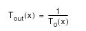
When computing the entries of T_out, the rules summarized in the following table are applied. The notation T₀(x-) and T₀(x+) refers to the ordinate values of the entries immediately preceding and following the entry whose ordinate value is being inverted.
Table 147: Entry Calculation Rules for Reciprocal Filter
| T₀(x) | T₀(x-) | T₀(x+) | T_out(x) |
|---|---|---|---|
 ¹ |
* | * | 1 / a |
| a = 0 | > 0 | > 0 | +infinity |
| a = 0 | > 0 | < 0 | +infinity undefined -infinity |
| a = 0 | < 0 | < 0 | -infinity |
| a = 0 | < 0 | > 0 | -infinity undefined +infinity |
| +infinity | * | * | 0.0 |
| -infinity | * | * | 0.0 |
| undefined | * | * | undefined |
Note 1: (a = real constant, * = any value)
Statistical Filters
Average Filter
The “average” filter is a unary filter used to operate on one input statistic T₀ to generate a second statistic, T_out, which represents the running mean of the ordinate values of T₀ beginning with the first entry.
Table 148: Synopsis of Average Filter
| Input Statistics | Parameters | Output |
|---|---|---|
| single input | none | running mean of ordinate values of input statistic |
The T_out statistic has the same number of entries as T₀ and the two statistics are aligned with each other with respect to the entries’ abscissa values. The ordinate value of the i-th T_out entry is computed as a function of all entries up to and including the i-th entry of T₀. Because there is not necessarily a one-to-one correspondence between the indices of the entries and their abscissa values, discrete notation is used in the following expression for the value of the n-th entry of T_out.
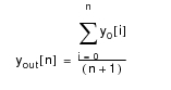
Note in the above expression that the denominator is the entry index plus one, due to the fact that entries are zero-indexed (in other words, n + 1 is the number of entries).
When using this filter, it is important to realize how special values such as +infinity, -infinity, and undefined are treated. If an undefined value is encountered in the input statistic a new entry is created at the same abscissa in T_out. If no defined entries precede this entry in T₀ then the new entry is marked as undefined in T_out as well; however, in the opposite case, the new entry is simply marked with the value of the preceding entry in T_out. In both cases, undefined entries are not considered part of the mean that is computed, and therefore their occurrence affects neither the numerator nor the denominator of the expression above. Therefore, a discrepancy between the expression for T_out and the actual algorithm of the filter can develop as undefined entries occur; a correction to this discrepancy can be made by subtracting from the denominator the number of undefined entries whose indices are less than or equal to n.
The first infinite value encountered in T₀ causes the value of T_out to become infinite as well (with same sign). The filter’s output will continue to be infinite for all remaining entries unless an infinite value of opposite sign is encountered at which point T_out will become undefined and remain so up to and including the final entry.
The following table lists the rules applied in computing the values of T_out. Because this filter incorporates the history of the input statistic into the calculation of each entry, the table relies on a variable Sₙ which is the sum of all defined entry ordinates of T₀ up to and including the n-th entry. In addition, the variable Uₙ is defined as the number of undefined entries in T₀ with index less than or equal to n.
Table 149: Entry Calculation Rules for Average Filter
| Sₙ₋₁ | T₀ | Uₙ₋₁ | Sₙ | Uₙ | T_out |
|---|---|---|---|---|---|
| a¹ | b | c | a + b | c | (a + b) / (n+1-c) |
| a | +infinity | c | +infinity | c | +infinity |
| a | -infinity | c | -infinity | c | -infinity |
| 0.0 | undefined | c = n | a | c+1 | undefined |
| a | undefined | c < n | a | c+1 | a / (n - c) |
| +infinity | b | c | +infinity | c | +infinity |
| +infinity | -infinity | c | undefined | c | undefined |
| -infinity | b | c | -infinity | c | -infinity |
| -infinity | +infinity | c | undefined | c | undefined |
| +infinity | undefined | c | +infinity | c+1 | +infinity |
| -infinity | undefined | c | -infinity | c+1 | -infinity |
| undefined | * | c | undefined | c or c+1 | undefined |
Note 1: (a, b, c = real constant, * = any value)
Time Average Filter
The “time_average” filter is a unary filter used to operate on one input statistic T₀ to generate a second statistic, T_out, which represents the running continuous average of the ordinate values of T₀ beginning with the first entry. The difference between this filter and the “mean” filter, described previously, is that entry values are not weighted equally, but are instead weighted by the difference between their own abscissa and that of the subsequent entry. The filter is named “time average” due to the fact that it is frequently applied to statistics whose horizontal axis represents time; however, it is also applicable to other types of statistics.
Table 150: Synopsis of Time Average Filter
| Input Statistics | Parameters | Output |
|---|---|---|
| single input | none | running continuous average of ordinate values of input statistic |
The T_out statistic has the same number of entries as T₀ and the two statistics are aligned with each other with respect to the entries’ abscissa values. The ordinate value of the i-th T_out entry is computed as a function of all entries up to and including the i-th entry of T₀. Because there is not necessarily a one-to-one correspondence between the indices of the entries and their abscissa values, discrete notation is used in the following expression for the value of the n-th entry of T_out.
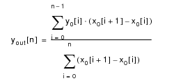
With regard to treatment of the special ordinate values +infinity, -infinity, and undefined, this filter behaves in a manner that is analogous to the “mean” filter, described earlier. In particular, undefined values are essentially ignored: the numerator of the above expression is not modified by their occurrence; and the width of an undefined interval does not contribute to the denominator term. Also, infinite ordinate values in the input statistic result infinite values of same sign for all subsequent entries of the output statistic. However, if infinite values of different sign are encountered, T_out becomes undefined. See Average Filter for a general understanding of how the time average filter is implemented.
Moving Average Filter
The “moving_average” filter is a unary filter used to operate on one input statistic T₀ to generate a second statistic, T_out, which represents the continuous average of the ordinate values of T₀ over intervals of a specified width. These intervals slide over the range of T₀’s abscissa so that T_out represents the average over the most recent interval. The interval width is set by the filter’s only parameter, which is called window.
Table 151: Synopsis of Moving Average Filter
| Input Statistics | Parameters | Output |
|---|---|---|
| single input | window: positive real number used to set averaging interval width | continuous average of input statistic ordinate values over most recent interval of width equal to “window” |
When the window parameter is set to a large value relative to the typical abscissa spacing between entries of the input statistic, the “moving_average” filter provides a smooth result that averages values together on a local basis. However, the window parameter may be selected to be any positive size, including extremely small values, making it possible for consecutive points to be more than one window apart. In such cases, the moving average should still exhibit change over the period of one window because it attempts to emulate a continuous averaging calculation. To improve the smoothness of its results, the “moving_average” filter may insert additional samples in the output statistic. Therefore, there is not necessarily a direct correspondence between the lengths of T₀ and T_out.
The normal value for the minimum abscissa distance is the value of min_dt/2, where min_dt equals minimum distance between abscissa points in the original statistic. This results in a given number of entries for the new statistic. The moving average filter limits the number of entries in the new statistic, however, to no more than 10 times the number of original entries. When this occurs, the x-axis increment is scaled up to result in a lower density of points on the x-axis and fewer points overall.
The general calculation of T_out’s values is quite complicated and involves many special cases for special undefined and infinite values. Due to the complexity of the algorithm, this manual does not present a full description, as was done for other predefined filters.
However, the following statements are useful to describe the filter’s behavior for most purposes:
- The “moving_average” filter’s computations are essentially composed of additions and multiplications of entry ordinates and abscissas. With regard to the special values for infinite and undefined entries, the same basic rules applied in other averaging filters are used, namely:
- Addition of two infinite values of same sign also yields an infinite value of same sign.
- Addition of two infinite values of opposite signs yields an undefined value.
- Undefined ordinate values in the input statistic are essentially ignored.
- Multiplication of an infinite value by a finite value yields an infinite value of appropriate sign.
- Given that the “moving_average” filter selects a new collection of abscissa points at which to compute the values of T_out, the following general expression represents the calculation performed by the filter. The expression shows that the moving average is calculated by integrating the input statistics over all the intervals that are included in a the window that extends from x_out[n] - W to x_out[n]. Because T_out and T₀ are not aligned, it is possible that the window’s boundaries do not coincide perfectly with entry abscissas in T₀. As a result, two additional terms are needed in the numerator to compute the contribution of these “partial” intervals. Note that because averaging is over a fixed window, the numerator is simply the constant that corresponds to the filter’s window parameter. As with other averaging filters, the general expression provided here is not precisely accurate in the case where undefined points appear in the input statistic.
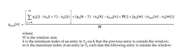
- The “moving_average” filter uses a backwards-looking integration. Therefore for an initial part of the output statistic, equal in abscissa span to the width of the window, the average value reflected in T_out will not be with respect to a full window, but rather with respect to a truncated window. This window grows progressively until it reaches the full size specified in the window parameter.
Sample Sum Filter
The “sample_sum” filter is a unary filter used to operate on one input statistic T₀ to generate a second statistic, T_out, which represents the running total of the ordinate values of T₀ beginning with the first entry.
Table 152: Synopsis of Sample Sum Filter
| Input Statistics | Parameters | Output |
|---|---|---|
| single input | none | running total of ordinate values of input statistic |
The T_out statistic has the same number of entries as T₀ and the two statistics are aligned with each other with respect to the entries’ abscissa values. The ordinate value of the i-th T_out entry is computed as a function of all entries up to and including the i-th entry of T₀. Because there is not necessarily a one-to-one correspondence between entries indices and abscissa values, discrete notation is used in the following expression for the value of the n-th entry of T_out.
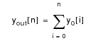
When using this filter, it is important to realize how special values such as +infinity, -infinity, and undefined are treated. If an undefined value is encountered in the input statistic, a new entry is created at the same abscissa in T_out. If no defined entries precede this entry in T₀ then the new entry is marked as undefined in T_out as well; however, in the opposite case, the new entry is simply marked with the value of the preceding entry in T_out. In both cases, undefined entries are not considered part of the sum that is computed, and therefore their occurrence is essentially ignored.
The first infinite value encountered in T₀ causes the value of T_out to become infinite as well (with same sign). The filter’s output will continue to be infinite for all remaining entries unless an infinite value of opposite sign is encountered, at which point T_out will become undefined and remain so up to and including the final entry.
The following table lists the rules applied in computing the values of T_out. Because this filter incorporates the history of the input statistic into the calculation of each entry, the table uses the previous value of T_out as an input appearing on the left side of the table. Note that the contents of the two left columns of the table can be interchanged to address symmetric cases.
Table 153: Entry Calculation Rules for Sample Sum Filter
| T_out[n-1] | T₀[n] | T_out[n] |
|---|---|---|
| a¹ | b | a + b |
| a | +infinity | +infinity |
| a | -infinity | -infinity |
| +infinity | -infinity | undefined |
| * | undefined | * (i.e., same) |
Note 1: (a, b = real constant, * = any value)
Calculus Operators and Related Analytical Filters
Differentiator Filter
The “differentiator” filter is a unary filter used to operate on one input statistic T₀ to generate a second statistic, T_out, which represents the derivative of T₀ with respect to its abscissa variable.
Table 154: Synopsis of Differentiator Filter
| Input Statistics | Parameters | Output |
|---|---|---|
| single input | none | single statistic representing the derivative of the input statistic with respect to its abscissa variable |
The derivative is computed using the forward differences in ordinate and abscissa. The ratio of these two quantities provides a correct value for the derivative over each interval, under the assumption that the statistic represents a continuous, piecewise linear function (i.e., the actual statistic behaves as shown when it is plotted with a linear draw style). If the statistic in fact represents a different type of continuous function, then this filter still provides an accurate estimate of the derivative, provided that the spacing between abscissa points is small. The calculation generally performed by the filter is the following (with the exception of entries that contain special values):
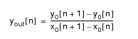
The input and output statistics are aligned with respect to the abscissa values of their entries. However, note that using the above expression, the “differentiator” filter is unable to compute a value for the final entry of the input statistic, because there is no following entry to calculate the required differences. Therefore, T_out is shorter than T₀ by one entry.
When computing the entries of T_out, the rules summarized in the following table are applied.
Table 155: Entry Calculation Rules for Differentiator Filter
| y₀[n+1] - y₀[n] | x₀[n+1] - x₀[n] | y_out[n] |
|---|---|---|
| a¹ |  |
a / b |
| a | ±infinity | 0.0 |
| * | 0 | undefined |
| undefined | * | undefined |
| * | undefined | undefined |
| +infinity | a > 0 | +infinity |
| +infinity | a < 0 | -infinity |
| -infinity | a > 0 | -infinity |
| -infinity | a < 0 | +infinity |
Note 1: (a, b = real constant, * = any value)
Integrator Filter
The “integrator” filter is a unary filter used to operate on one input statistic T₀ to generate a second statistic, T_out, which represents the integral of T₀ with respect to its abscissa variable.
Table 156: Synopsis of Integrator Filter
| Input Statistics | Parameters | Output |
|---|---|---|
| single input | none | single statistic representing the integral of the input statistic with respect to its abscissa variable |
The integral statistic is computed as the area under the input statistic using the “sample-and-hold” interpretation of the statistic. In other words, the area between the statistic and the horizontal axis is obtained for a particular entry by multiplying the width of the abscissa interval until the next entry by the ordinate value of the entry. The calculation generally performed by the filter is the following (with the exception of special handling for entries that contain special values):
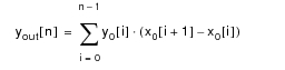
The input and output statistics are aligned with respect to the abscissa values of their entries. The output statistic may have one additional entry relative to the input statistic to account for the area contributed by the final entry of the latter. This depends upon whether the input statistic’s end-of-statistic marker has an abscissa that exceeds that of the final entry with an ordinary value.
The “integrator” filter treats special values much in the same way as other accumulating filters such as the “mean”, “time_average”, and “sample_sum” filters. That is primarily to say adding infinite values of opposite sign yields an undefined value, and that adding undefined entries in the input statistic are essentially ignored (i.e., in this case, these entries are treated as though their ordinate value were zero sine they contribute nothing to the integral). The following table lists the rules applied in computing the values of T_out. Because this filter incorporates the history of the input statistic into the calculation of each entry, the table uses the previous value of T_out as an input appearing on the left side of the table. Note that the contents of the two left columns of the table can be interchanged to address symmetric cases.
Table 157: Entry Calculation Rules for Integrator Filter
| y_out[n-1] | y₀[n-1] | x₀[n] - x₀[n-1] | y_out[n] |
|---|---|---|---|
| a¹ | b | c | a + bc |
| a | ±infinity | c | ±infinity |
| a | undefined | c | a |
| +infinity | b | c | +infinity |
| -infinity | b | c | -infinity |
| +infinity | -infinity | c | undefined |
| -infinity | +infinity | c | undefined |
| undefined | * | c | undefined |
Note 1: (a, b, c = real constant, * = any value)
Exponentiator Filter
The “exponentiator” filter is a unary filter used to operate on one input statistic T₀ to generate a second statistic, T_out, which is obtained by raising the ordinate values in T₀ to a fixed power. This power value is designated via the filter’s single parameter called exponent.
Table 158: Synopsis of Exponentiator Filter
| Input Statistics | Parameters | Output |
|---|---|---|
| single input | exponent: real number used as “power” of exponentiation | single statistic composed of values of input statistic raised to the power of exponent |
Because special manipulations might be required to handle undefined points in T_out and indeterminate forms, the resulting statistic might not have the exact same length as the input statistic. In particular, when the specified exponent is negative, additional points might have to be inserted. For more information, see Reciprocal Filter.
In general however, the T_out statistic has a set of entries with abscissa values that match those of T₀. For entries where the exponentiation result is defined, the relationship between input and output statistic is given by the following:

The following table lists the rules applied in the computation of the entries of T_out in the case where the exponent is positive or zero. For cases where the exponent is negative, this table can be used to determine an intermediate result and subsequently, the calculation rules of the reciprocal filter can be applied.
Table 159: Entry Calculation Rules for Exponent Filter (with Nonnegative or Infinite Exponent)
| T₀(x) | exponent | T_out(x) |
|---|---|---|
 ¹ |
 |
a^b |
| a < 0 | b | a^b |
| a < 0 | b non-integer | undefined |
| a > 1.0 | -infinity | 0.0 |
| a > 1.0 | +infinity | +infinity |
| a = 1.0 | ±infinity | 1.0 |
| a < 1.0 | +infinity | 0.0 |
| a < 1.0 | -infinity | +infinity |
| a < 0 | ±infinity | undefined |
| ±infinity | 0.0 | 1.0 |
| +infinity | b > 0.0 | +infinity |
| -infinity |  |
+infinity |
| -infinity | b odd integer | -infinity |
| +infinity | +infinity | +infinity |
| +infinity | -infinity | undefined |
| -infinity | b non-integer | undefined |
| -infinity | +infinity | undefined |
Note 1: (a, b = real constant, * = any value)
Logarithm Filter
The “logarithm” filter is a unary filter used to operate on one input statistic T₀ to generate a second statistic, T_out, which is obtained by computing the base ten logarithm, or common logarithm, of the ordinate entries of T₀.
Table 160: Synopsis of Logarithm Filter
| Input Statistics | Parameters | Output |
|---|---|---|
| single input | none | single statistic composed of base 10 logarithms of values of input statistic |
The number of entries in the T_out statistic is identical to that of T₀ and the entries of both statistics are aligned with each other on the horizontal axis. The logarithm function is not defined for all values, meaning that some entries with special values may be present in T_out. However, for entries where the logarithm result is defined, the relationship between input and output statistic is given by the following:

The following table lists the rules applied in the computation of the entries of T_out.
Table 161: Entry Calculation Rules for Logarithm Filter
| T₀(x) | T_out(x) |
|---|---|
| a > 0.0¹ | log₁₀(a) |
| a = 0.0 | -infinity |
| a < 0.0 | undefined |
| +infinity | +infinity |
| -infinity | undefined |
| undefined | undefined |
Note 1: (a = real constant, * = any value)
Miscellaneous Filters
Abscissa Filter
The “abscissa” filter is a unary filter used to operate on one input statistic T₀ to generate a second statistic, T_out, whose ordinate values are simply the abscissa values of the entries of T₀.
Table 162: Synopsis of Abscissa Filter
| Input Statistics | Parameters | Output |
|---|---|---|
| single input | none | single statistic composed of abscissa values of input statistic |
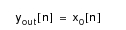
The number of entries in the T_out statistic is identical to that of T₀ and the entries of both statistics are aligned with each other on the horizontal axis. Note that only the abscissa values of the input statistic are relevant to the computation performed by this filter, as shown in the following equation relating input and output statistics.
Delay Element Filter
The “delay_element” filter is a unary filter used to operate on one input statistic T₀ to generate a second statistic, T_out, which is obtained by translating T₀ along the horizontal axis by a fixed amount. The translation distance is controlled by the sole parameter of the filter, called delay. A positive value for delay causes a translation of the statistic in the positive abscissa direction.
Table 163: Synopsis of Delay Element Filter
| Input Statistics | Parameters | Output |
|---|---|---|
| single input | Delay: amount to shift statistic | single statistic composed of same entries as input statistic shifted in abscissa direction |
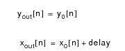
The length of T₀ and T_out are identical, with the entries of T_out computed as follows (note: all special values are simply translated to new abscissas).
Glitch Notch Filter
The “glitch_notch” filter is a unary filter used to operate on one input statistic T₀ to generate a second statistic, T_out, by eliminating the occurrence of multiple entries that share the same abscissa value (such an occurrence is referred to as a glitch). T_out is constructed by copying entries from T₀. However, if a sequence of consecutive entries (at least two) with the same abscissa is encountered in T₀, all but the last entry in this sequence are ignored, and the last entry is copied into T_out. Therefore, T_out is glitch-free.
Table 164: Synopsis of Glitch Notch Filter
| Input Statistics | Parameters | Output |
|---|---|---|
| single input | none | single statistic composed of same entries as input statistic but with at most one entry at each distinct abscissa |
Because the purpose of this filter is to eliminate entries to ensure uniqueness of entries at each abscissa value, the length of T_out might be less than that of T₀. If no glitches exist in T₀, then T_out is simply an identical copy of T₀.
Limiter Filter
The “limiter” filter is a unary filter used to operate on one input statistic T₀ to generate a second statistic, T_out, which is obtained by constraining the ordinate values T₀ within a specified range. The lower and upper limits of this range are controlled by the filter parameters called min_val and max_val, respectively. These are inclusive bounds for the range.
The “limiter” filter performs a transformation on T₀ by copying entries into T_out and simultaneously clipping them to ensure that they are within the specified interval. Entries whose ordinate values exceed max_val are modified to have the value max_val. Similarly, entries whose ordinate values are less than min_val are modified to have the value min_val.
Table 165: Synopsis of Limiter Filter
| Input Statistics | Parameters | Output |
|---|---|---|
| single input | Min_val: lower bound of vertical range Max_val: upper bound of vertical range |
single statistic composed of same entries as input statistic, but constrained within the specified range [min_val, max_val] |
The length of T₀ and T_out are identical, and are aligned with each other along the horizontal axis. The entries of T_out are computed as shown below. Undefined entries are not transformed by this filter. Positive infinite ordinates are clipped to the upper bound, and negative infinite ordinates are clipped to the lower bound.

Time Window Filter
The “time_window” filter is a unary filter used to operate on one input statistic T₀ to generate a second statistic, T_out, which is obtained by eliminating all entries whose abscissa values lie outside a specified range. The lower and upper limits of this range are controlled by the filter parameters called min_time and max_time, respectively. These bounds themselves are also included in the range. The names min_time and max_time are used due to the fact that this filter is frequently applied to statistics and/or output vectors that use time as their abscissa variable. However, the “time window” filter is equally applicable to other types of statistics.
The “time_window” filter performs a transformation on T₀ by copying only those entries into T_out that have abscissa variables within the specified range. Entries whose abscissa values exceed max_time are discarded, as are those whose abscissa values are less than min_time. Other entries are copied into T_out unmodified.
Table 166: Synopsis of Time Window Filter
| Input Statistics | Parameters | Output |
|---|---|---|
| single input | Min_time: lower bound of horizontal range Max_time: upper bound of horizontal range |
single statistic composed of only those entries in T₀ whose abscissa values are in the inclusive range [min_val, max_val] |
Value Notch Filter
The “value_notch” filter is a unary filter used to operate on one input statistic T₀ to generate a second statistic, T_out. T_out is obtained by eliminating all entries that are approximately equal to the parameter value. “Approximately equal” is defined as falling within a range determined by a specified ordinate value (x) and the value of the “value_notch_filter_tolerance” preference (tol). If T₀ is greater than x - tol and less than x + tol, it is eliminated; otherwise T₀ is simply copied to the output statistic T_out. (“value_notch_filter_tolerance” has a default value of 10⁻⁹.)
Table 167: Synopsis of Value Notch Filter
| Input Statistics | Parameters | Output |
|---|---|---|
| single input | value: entries with this ordinate value are eliminated | single statistic composed of only those entries in T₀ whose ordinate values are higher or lower than the specified value by a certain number, defined by the “value_notch_filter_tolerance” preference |