Histograms and Probability Profiles
Five operations are provided for the purpose of establishing a distribution of a sample set of collected values:
- Probability Density (PDF)
- Cumulative Distribution (CDF)
- Probability Mass (PMF)
- Histogram (Sample-Distribution)
- Histogram (Time-Distribution)
- Scatter Plot (Time-Join)
Each operation is unary (i.e., requires only one statistic as input) and produces a new single-statistic panel to hold its result when it completes. The computations done by each of these operations are described in this section. See “Project Editor” on page 89 for instructions on their use.
Probability Density Function
The probability density function (PDF) operation can be thought of as a continuous equivalent of the PMF described earlier. Like probability mass, probability density corresponds to the likelihood that the input statistic’s ordinate lies within a specific range; however, density is evaluated proportionally to the interval of interest. Therefore, if the statistic’s ordinate value has a likelihood 0.1 of falling in a given interval with width d, and also has a likelihood 0.1 of falling in a second interval with width d/2, then the probability density in the second interval is twice as high. In other words, probability density is highest when a small set of possible values has a high associated probability mass.
The actual definition of a probability density function is based on the fact that its integral over a given interval yields the probability mass associated with that interval. The probability mass associated with an interval can also be obtained by computing the difference in the CDF for the upper and lower limits of the interval. As interval widths become infinitesimally small, it can be seen that the PDF is therefore the derivative of the CDF with respect to the outcome (i.e., ordinate) variable.
The relationship between a PDF and a CDF is in fact the basis for the method used by the Results Browser to compute PDFs. A CDF is first computed as described earlier in this section, and a differentiation is performed to construct a PDF. Because the original statistic data is necessarily discrete, differentiation is performed in an approximate manner by dividing probability mass associated with an interval by the interval’s width. In other words, the difference between two consecutive CDF values is divided by the difference in the corresponding ordinates. The resulting value is taken as the density associated with the interval and is placed at the interval’s lower limit. Therefore if a statistic contains two consecutive ordinate values y1, and y2, the PDF is computed as follows:
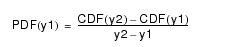
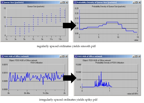
An immediate consequence of this computation method is that PDFs can have extremely large values when the input statistic has distinct but closely spaced ordinate values, because the (y2 - y1) difference becomes small. Therefore, if input statistic ordinate values are unevenly spaced (i.e., some very small differences exist, but also some significantly larger ones), PDFs can have a “spiky” or discontinuous appearance, with certain density values dwarfing others. In such cases, PDFs tend not to be as useful as the PMF or histogram operations.
A second consequence of this calculation is that the PDF contains one less entry than the CDF due to the fact that no forward-looking difference can be calculated for the final (i.e., maximum) ordinate value.
Finally, the integral of the PDF statistic, which can be computed using the correct filter, produces a statistic that is identical to the CDF in its shape. However, the initial value of the CDF is lost in computing the PDF, meaning that the two statistics differ by a constant. This difference is particularly noticeable when the original statistic has a small number of distinct ordinate values, because the CDFs value for the minimum ordinate is at least the reciprocal of this number (i.e., this is the probability mass associated with the first ordinate value).
Figure 283: Results of PDF Operation for Regularly and Irregularly Spaced Ordinates
Cumulative Distribution Function
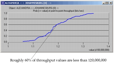
Like the probability mass function, the cumulative distribution function (CDF) of a statistic relates to the likelihood of occurrence of the statistic’s ordinate values. However, rather than provide the probability mass of each ordinate’s occurrence, the CDF shows the accumulated probability mass of all ordinates less than or equal to a particular ordinate, hence the term “cumulative”. This form of presentation is useful when particular ordinate value thresholds are of interest. For example, it may be of interest to determine the likelihood of receiving a message whose delays exceeds a particular value, because under such conditions, the packet can not be of any practical use. In fact in many cases, system performance requirements are stated in terms of maximum tolerances for such probabilities; i.e., “the probability of receiving a packet with delay >= 20 ms must be no greater than 0.1”. The CDFs resulting statistic allows compliance with such a requirement to be readily determined by finding the threshold value on the horizontal axis and the corresponding probability on the vertical axis. In the example of this paragraph, a compliant system would be characterized by a CDF value of at least 0.90 at the 20 ms abscissa position. A possible CDF is shown below for a non-compliant system under the conditions of this example.
Figure 284: Using a CDF to Determine Proportion of Entries below a Threshold
The computation of a CDF resembles that of a PMF in the sense that proportions for each ordinate value in the original statistic are computed. The same weight, which is the reciprocal of the number of entries, is attributed to each entry. Therefore if there are 100 entries, then each entry has a weight of 0.01, and if there are five entries whose ordinate values is y, then the ordinate y has a total probability mass of 0.05. The entries of the CDF are constructed by positioning the distinct ordinate values of the original statistic in increasing order on the abscissa, with one entry for each such value. The CDF value for the initial entry is simply the probability mass of the corresponding ordinate. The CDF value for the second entry is equal to the CDF value of the first entry augmented by the probability mass of its corresponding ordinate value, and so on. The CDF is essentially a running sum of the values of the PMF.
Two simple properties of the CDF result from the method of computation described above: (1) because each CDF value is computed by adding a positive probability mass to the previous value, CDFs are monotonically increasing; (2) because the sum of all probability masses must add up to unity, all CDFs must have a final value of 1.0; this also makes sense under the definition of the CDF, because one would expect the likelihood of obtaining an ordinate value less than or equal to the maximum ordinate value to simply be 1.0.
Probability Mass Function
The Probability Mass Function (PMF) operation allows the distribution of a statistic’s ordinate values to be obtained, much in the same manner as a sample-distribution histogram. While PMFs do count entries to measure the frequency with which ordinate values occur, counters are not maintained on a per-interval basis. Instead, each distinct ordinate value is counted separately, so that only entries with the exact same ordinate can combine to produce higher PMF values.
The counters used by the PMF operation to compute the frequency of each ordinate value are normalized with respect to the total number of entries in the original statistic. In other words, the resulting PMF represents the frequency of occurrence of a particular ordinate value as a proportion of the number of occurrences of all ordinate values. Therefore, the measurement provided by a PMF can be though of as the likelihood that an entry chosen at random among all the entries of the original statistic, would have a particular ordinate value. For such a selection experiment, the likelihood of choosing a particular ordinate value is also sometimes called the probability mass of that outcome, hence the name of the operation.
The following set of data, and the accompanying statistic, illustrate the calculation of a PMF.
Figure 285: Calculation of Probability Mass Function
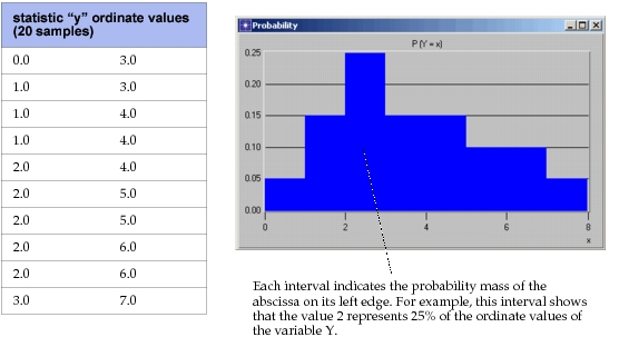
The fact that distinct ordinate values are not aggregated on the basis of intervals makes PMFs appropriate to apply to statistics that contain a relatively small number of discrete ordinate values. In such cases, sample-distribution histograms may be less appropriate than PMFs due to one primary problem: if the discrete values that are present are unevenly spaced, it may be difficult to choose a histogram interval width that provides for both good separation of the values and a reasonable number of intervals. For example, consider a statistic containing the three ordinate values 0.0, 0.001, and 1000.0. To treat the values distinctly, a sample-distribution histogram would require an interval width that is the smallest difference between consecutive values, or in this case 0.001. However, the highest value, 1000.0, can only be encompassed with one million intervals in this case, causing the sample-distribution histogram to produce an extremely large statistic.
Conversely, PMFs may not provide significant insight into the characteristics of statistics containing a very diverse set of ordinate values. This is due to the fact that each ordinate value is separately counted and that as a result, little can be said about which ordinate region(s) exhibit the highest density in terms of the statistic’s presence. In the extreme case, if each value in the original statistic is unique, then the resulting PMF will have a constant value of 1.0, providing almost no visually apparent information on the distribution of the values.
Histogram (Sample-Distribution)
The sample-distribution histogram of a statistic reflects the distribution of its ordinate values over evenly spaced intervals of the vertical axis. The vertical axis is divided into N distinct intervals beginning at the lower bound and ending at the upper bound. By default, N is 100, but this value may vary according to a user-selected interval width. For each interval, the Sample-Distribution Histogram operation then creates and initializes a separate counter to represent the frequency with which entries occur in that interval. Subsequently, the entire statistic is traversed and each entry analyzed; the counter whose interval contains the entry’s ordinate value is incremented by one.
The statistic that results from this operation contains N entries corresponding to the N intervals; because these intervals divide the vertical axis of the original statistic, they appear on the horizontal axis of the new statistic, and the vertical axis corresponds to the frequencies of occurrence held in the N counters. Note from the description of this computation, that abscissa values in the original statistic are not relevant to the sample-distribution histogram. As an example, consider computing a histogram for the following set of entries:
| abscissa “x” | ordinate “y” |
|---|---|
| 1.0 | 1.0 |
| 2.0 | 4.0 |
| 3.0 | 1.0 |
| 4.0 | 2.0 |
| 5.0 | 1.0 |
| 6.0 | 3.0 |
| 7.0 | 4.0 |
| 8.0 | 6.0 |
| 9.0 | 1.0 |
| 10.0 | 0.0 |
The ordinate values of this statistic range from 0.0 to 6.0 and are all integers. The default setting of 100 intervals would create far more intervals than there are values, yielding an essentially empty histogram. An interval size of 1.0 is more sensible. The counting process performed by the sample-distribution histogram table is summarized by the table below. Notice that intervals are inclusive of their lower bound, but not of their upper bound, so that they provide a complete partitioning of the vertical axis within its range, but do not overlap with each other.
| Interval | Frequency of Occurrence |
|---|---|
| 0.0 <= y < 1.0 | 1 |
| 1.0 <= y < 2.0 | 4 |
| 2.0 <= y < 3.0 | 1 |
| 3.0 <= y < 4.0 | 1 |
| 4.0 <= y < 5.0 | 2 |
| 5.0 <= y < 6.0 | 0 |
| 6.0 <= y < 7.0 | 1 |
The statistic resulting from the sample-distribution histogram operation is easily obtained from the frequency table above. The “y” label now appears on the horizontal axis and the vertical axis measures the frequency of occurrence. The profile of the histogram indicates the degree to which regions of the variable y’s range are occupied by the original statistic. In general, this is viewed as directly related to the likelihood that a randomly selected sample of the variable y will fall within a particular interval. This is illustrated for the example data set shown in the following figure.
Figure 286: Sample-Distribution Histogram for Y variable
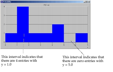
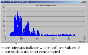
For more complex input statistics containing a richer set of ordinate values, sample-distribution histograms can be interpreted as a density profile, showing where the ordinate values are concentrated.
The following figure shows this interpretation of the sample-distribution histogram.
Figure 287: Sample-Distribution Histogram Showing Density Profile of Input Statistic
Histogram (Time-Distribution)
Time-distribution histograms resemble sample-distribution histograms in the sense that they establish a profile for the ordinate value of a statistic. The resulting profile shows how frequently the ordinate value of the statistic lies within specific ranges. Therefore, this operation divides the vertical axis into intervals in the same manner as the sample-distribution histogram. However, rather than use the number of entries falling within each interval as the measure of frequency, a time-distribution histogram is based on the “time spent” by the statistic within the intervals. In other words, ordinate values are still the basis for the histogram, but weighting of each entry is performed differently: sample-distribution histograms weight each entry with a coefficient of 1.0; time-distribution histograms weight each entry with the difference between its abscissa value and the abscissa value of the next entry.
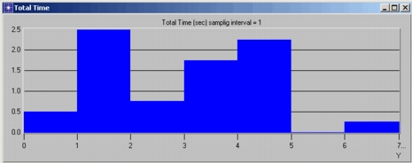
Time-distribution histograms are computed in much the same way as sample-distribution histograms, except that for each interval, an accumulator is used to total the abscissa interval widths. The following example shows the computation procedure for a specific set of data. Note that the ordinate values are identical to those used in the example for the sample-distribution histogram in the previous section; only the abscissas are changed. Because sample-distribution histograms are not sensitive to abscissa values, the result for this statistic would be identical to the one shown in the previous section. Therefore, the result shown here can be used to contrast the behavior of the two histogram methods.
| abscissa “x” | ordinate “y” |
|---|---|
| 1.0 | 1.0 |
| 1.5 | 4.0 |
| 3.0 | 1.0 |
| 3.25 | 2.0 |
| 4.0 | 1.0 |
| 5.25 | 3.0 |
| 7.0 | 4.0 |
| 7.75 | 6.0 |
| 8.0 | 1.0 |
| 8.5 | 0.0 |
| 9.0 | end-of-statistic |
The ordinate values of this statistic range from 0.0 to 6.0 and are all integers. The default setting of 100 intervals would create far more intervals than there are values, yielding an essentially empty histogram. An interval size of 1.0 is therefore more sensible. The calculation performed by the time-distribution histogram table is summarized by the table below. For each interval an accumulator variable is maintained to compute the total abscissa span for which the statistic’s ordinate falls within the interval. Notice that intervals are inclusive of their lower bound, but not of their upper bound, so that they provide a complete partitioning of the vertical axis within its range, but do not overlap with each other.
| Interval | abscissa-span accumulator |
|---|---|
| 0.0 <= y < 1.0 | 0.5 |
| 1.0 <= y < 2.0 | 2.5 |
| 2.0 <= y < 3.0 | 0.75 |
| 3.0 <= y < 4.0 | 1.75 |
| 4.0 <= y < 5.0 | 2.25 |
| 5.0 <= y < 6.0 | 0.0 |
| 6.0 <= y < 7.0 | 0.25 |
Figure 288: Time-Distribution Histogram for Y Variable
Comparing Time-Distribution and Sample-Distribution Histograms
For certain input statistics, a time-distribution histogram yields results that have a very similar profile to a sample-distribution histogram. In particular, for input statistics that have regularly spaced entries in terms of abscissa values, such as the example in the previous section, the shapes of the two histograms are identical (note that the values shown in the histogram are not necessarily identical because abscissa values may be spaced by a value other than 1.0). However, for cases where abscissa values of entries are not regularly spaced, results can vary significantly between the two methods.
In general, a time-distribution histogram is most appropriate for statistics that measure a quantity representing state information. For these types of quantities, the entries of the statistic are merely samples of a statistic that is defined at all times. Examples of such quantities include the size of a queue, and the average utilization of a channel, both measured over time. In the case of queue size, the time-distribution histogram represents the amount of time that the queue size actually holds a particular value, or falls within a range of values; similarly, for average channel utilization, a time-distribution histogram indicates the total duration during which this statistic falls in the selected intervals.
In contrast, sample-distribution histograms are more appropriate for instantaneously measured quantities such as delays associated with received messages, and error rates in transmitted packets. These statistics tend to characterize the occurrence of particular events, whose frequency of occurrence can be counted. Therefore, the sample-distribution histogram is useful to indicate how many messages experienced a particular level of delay, regardless of when these delays were measured. However, a sample-distribution histogram applied to a queue size statistic actually only indicates how many times the queue size changed to then arrive at a particular new size; this provides no definite information about how often one might expect to find the queue at a particular size.
Scatter Plot (Time-Join)
The time-join operation of the Results Browser accepts two statistics and/or vectors as inputs to create a new statistic that shows the relationship (or lack thereof) between them. The ordinate variable of the first statistic that is selected becomes the abscissa variable of the new statistic; the ordinate variable of the second statistic is mapped into the ordinate variable of the new statistic. The abscissa variable of both statistics is assumed (but not verified) to be the same and becomes the implicit parameter used to relate the two input statistics.
This operation uses a simple mechanism to create the entries of the new statistic. For each entry in the first statistic, an entry with equal abscissa is searched for in the second statistic; if no exact match is found, then the nearest entry with a lesser abscissa value is selected. The ordinate values of each of this pair of entries is used to form an entry for the new statistic (i.e., the ordinate of the first entry becomes the abscissa of the new entry, and the ordinate of the second entry becomes the ordinate of the new entry).
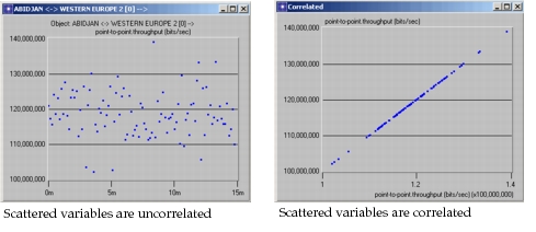
The scatter plot statistic that results from this operation shows a possible correlation between the two input statistics based on their abscissa variables. In general, the resulting statistic is viewed using the discrete draw style and appears as a cloud of points. If the cloud appears relatively shapeless with many ordinates for each abscissa, and vice versa, then it can be assumed that there is no strong correlation between the two input statistics. Otherwise, the scatter plot statistic provides a mapping indicating either a dependency between the ordinate variables of the two input statistics, or a correlated dependency on one or more other factors. The following scatter plots provide examples of the operation’s result for correlated and uncorrelated pairs of input statistics.
Figure 289: Examples of Scatter Plots