Data Presentation
The Results Browser offers a number of options with regard to the graphical presentation of a panel. These options never affect the data content of the panel, but only the manner in which the data is displayed. Access to the presentation options is via the Edit Panel Properties and Edit Graph Properties operations, which are activated by clicking with the right mouse button while the cursor is in a panel or graph, respectively.
Graphs
The graphs shown previously in this section show analysis panels that contain one graph. An analysis panel can have more than one graph, however, so long as all graphs can share the same horizontal axis. While the vertical axes may differ in a panel, all graphs in a panel must be able to use the same horizontal axis. Because of this, separate graphs in an analysis panel stack vertically, as shown in the following figure.
Figure 271: Two Graphs In One Analysis Panel
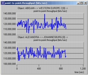
You can create a panel with multiple graphs or add graphs to the analysis panel later.
Panels
Graphs reside in an analysis panel. Clicking in the panel, as opposed to a graph, brings up the Edit Panel Properties dialog box, which allows the appearance of the horizontal axis to be changed or the draw style for all statistics in the graph to be globally set. The Statistics Info operation provides useful information about the statistics contained in the panel, including the data points themselves. The Edit Panel Properties dialog box also allows additional graphs to be added to the panel.
Drawing Style
Each graph within a panel can be assigned one of five possible graphical representations, called the graph's draw style. Each graph's draw style is controlled independently of the draw styles of other graphs. The drawing styles include discrete, linear, sample-hold, bar, bar chart, and square-wave.
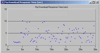
The discrete draw style provides the most direct view of the actual data content because one "dot" is used to represent each entry in the statistic (provided that the ordinate is not undefined). Because no attempt is made to attribute ordinate values to intermediate abscissa values, as is intrinsically done by the other draw styles, the discrete drawing style is most appropriate for graphs that represent a set of independent samples where intermediate values are not well defined. For example, a typical statistic resulting from measuring end-to-end delay for each received packet at the time where it is received is plotted below. Though it may be of interest in some cases to use the linear draw style to emphasize a trend in the discrete points, estimating the delay value at times between the packet arrivals does not correspond to a measurement that could actually be taken.
Figure 272: Statistic Plotted using Discrete Draw Style
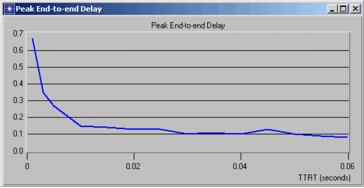
The linear draw style consists of drawing line segments between the points that are defined by a statistic's entries. One of the uses of this style is to represent intermediate points for which the statistic contains no samples, but which can be assumed to exist nonetheless. A common example of this is for panels containing scalar data, where each point represents the result collected by a simulation; the linear draw style can be used to "fill in" or approximate parts of the curve that lie between available data points, as shown in the following example.
Figure 273: Scalar Data Plotted with Linear Draw Style
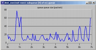
Because the resulting graph is without breaks (except at undefined points), the linear draw style is also sometimes used simply to emphasize the trend in a statistic, even if the statistic is discrete in nature. An example of this is shown in the second panel below, which contains the statistic for the size of a queue (i.e., the number of packets it contains) as it varies over time.
Figure 274: Discrete Variable Plotted Using Linear Draw Style
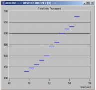
The sample-hold draw style is based on the notion that between abscissa values, no new information is known about certain types of statistics, and therefore these statistics should be assumed to maintain their previous ordinate value. This interpretation of a statistic's discrete set of entries makes sense for many statistics collected in Modeler-based simulations. Any statistic that represents a counter of some type, such as a queue size, the number of packets received without errors, or the number of times a queue has overflowed, inherently maintains its value until a new sample is obtained.
Figure 275: Counter Variable Plotted Using Sample-Hold Draw Style
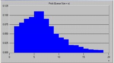
The bar draw style is essentially a simple extension of the sample-hold draw style, where the horizontal segment that is drawn at each entry is instead extended into a filled in bar that reaches down to the horizontal axis. This is the traditional "bar chart" which is useful for expressing the weight associated with each recorded abscissa value. This style is therefore often used to represent histogram data and probability distributions.
Figure 276: Probability Distribution Plotted Using Bar Draw Style
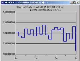
The square wave draw style is similar to both the sample-hold draw style and the bar draw style. It is, in effect, a bar graph that is not filled in. Vertical lines connect each horizontal segment, but the horizontal segments do not extend to the abscissa.
Figure 277: Data Plotted Using Square Wave Draw Style