Computing Confidence in Simulation Results
As explained in Chapter 10 "Simulation Design" on page 375, system models that include stochastic behavior have results that are dependent on the initial seeding of the random number generator. Because a particular random seed selection can potentially result in an anomalous, or non-representative behavior, it is important for each model configuration to be exercised with several random number seeds, to be able to determine standard, or typical behavior. The basic principle applied here is that if a typical behavior exists, and if many independent trials are performed, it is likely that a significant majority of these trials will fall within a close range of the standard.
One of the important issues a simulation designer must confront, when performing simulations incorporating stochastic processes, is that of deciding how many separately seeded trials to run to have sufficient data to make a statement about the system's typical behavior. Of course, the simulation designer can never be absolutely certain that the results obtained are representative, because it is possible to be "unlucky" in the sense that all, or most of the chosen random seeds could lead to anomalous behavior. However, as more seeds are chosen, the possibility of this happening becomes more remote, particularly because after all, standard behavior should be observed more frequently than anomalous behavior. This leads to the notion of attempting to achieve a certain level of confidence in the results obtained from a simulation study, by ensuring that a sufficient number of simulations are performed.
Confidence Intervals
The field of statistics provides methods for calculating confidence in an estimate, based on a trial or series of random trials. The techniques that it provides are also frequently used in applied sciences where field measurements are subject to error, and multiple measurements are taken to attempt to place a bound on the magnitude of that error. The Results Browser provides a basic capability in this area by automatically calculating and displaying confidence intervals for statistics already contained within panels. This capability is supported by the Show Confidence Interval checkbox in the Edit Graph Properties dialog box.
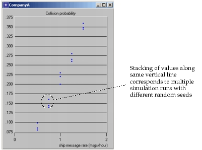
The confidence intervals calculated by the Results Browser are for the mean ordinate value of a set of entries. For the purposes of this operation, entry sets are defined by collocation at the same abscissa. This approach to calculating confidence intervals is designed primarily to support confidence estimation for scalar data collected in multi-seed parametric experiments, where one or more input parameters are varied, and for each input parameter value, multiple random number seeds are used to obtain multiple output parameters. The type of statistics that result from this type of simulation study (prior to confidence interval calculation) are illustrated by the example below. The vertical "columns" of entries correspond to the multiple experiments run by varying the random seed and maintaining a fixed value for an input parameter.
Figure 279: Statistic Consisting of Scalar Data from Multiple Simulation Runs
Suppose that a number of simulations of a system have been run with different random number seeds to obtain N samples of the statistic X. Even though X may take on many values, and X's precise distribution is unknown, it is possible to define a value μ, which is the true mean of the random variable X. One way to think of μ is as the mean value of an extremely large set of samples of X, if it were possible to run such a large number of simulations to obtain this sample set. The reason μ is interesting as the true mean of X is that it represents the typical behavior of the modeled system with regard to the statistic X.
Because it is not usually possible to run a very large number of simulations to determine μ (theoretically, an infinite number would be required), it is interesting to determine the degree of precision with which the mean value  of an N-sample set approximates μ. This determines whether the value
 can be used with confidence to make statements about the typical behavior of the modeled system.
The fundamental principle used in establishing confidence in an  measurement is called the central limit theorem. To understand this theorem, consider the experiment consisting in the collection of N samples of X, and the calculation of the average value
 of the N samples; in other words,
 is considered to be the result of one trial of the experiment. Then consider that this experiment may be performed many times, and that the resulting statistic
 has its own distribution. The central limit theorem states that regardless of X's actual distribution (this is an important generalization, because very little may be known about X), as the number of samples N grows large, the random variable
 has a distribution that approaches that of a normal random variable with mean μ, the same mean as the random variable X itself. The theorem further states that if the true variance of X is
 , then the variance of the statistic
 is
 .
The utility of this theorem, with respect to establishing confidence in a measurement, lies in the fact that if sufficient samples are taken, a normal distribution (which has known properties) can be worked with, rather than the unknown distribution of X. Assuming that a sufficient sample size N has been chosen, the sample  of the variable
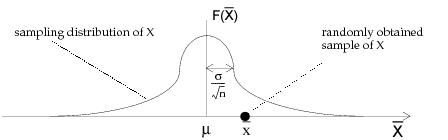
 taken from a sequence of simulations can be placed on the hypothetical sampling distribution of
 as shown below.
Figure 280: Sampling Distribution of 
Because the distribution of  is normal, the probability that the random sample
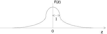
 falls within a particular distance of μ can be computed. Usually this distance is measured in terms of the number of standard deviations that separate the random sample from the mean. This way, a "standardized normal variable"
 is defined, for which the standard deviation is unity and the mean is zero, as shown below.
Figure 281: Sampling Distribution of 
If the positive value z_α is defined such that Prob (-z_α < z < z_α) = α, then the following statement can be made by substituting for z (note: most standard statistics textbooks provide tables mapping α to z_α, or equivalent variables). This statement can simply be thought of as defining the probability that  is within a particular distance of μ, based on the fact that the distribution of
 is normal.
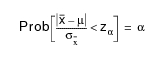
Conversely, this statement can be thought of as assigning a probability to the condition that the true mean μ is within a particular distance of the random sample  , as shown below (note that the standard deviation of
 is expressed in terms of the standard deviation of X, based on the central limit theorem).
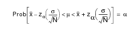
This statement introduces the notion of a confidence interval for μ, which is defined to be the interval of real numbers [Θ_L, Θ_R], such that the probability that μ lies within this interval has a particular value α. This interval is referred to as the 100α percent confidence interval for μ. In other words, if α = 0.95, the interval is called the 95% confidence interval for μ, because there is a 95% certainty level that the true mean of X lies within the interval's bounds. It is clear from the preceding inequalities that the confidence interval limits can be expressed as follows:

From these definitions, it is clear that the confidence interval widens as the degree of confidence increases; this makes sense, because to achieve a high level of confidence that the true mean is within a particular interval, one can expect to make a less restrictive hypothesis about that interval; similarly, if one is willing to accept a lower degree of confidence, a more constraining hypothesis can be made about the interval. As an extreme example, one can be 100% confident that the value μ lies between negative and positive infinity. In practice, a few particular confidence levels are chosen as shown in the following table.
Table 136: Selected Confidence Levels
| confidence level α | z_α |
|---|---|
| 99% | 2.575 |
| 98% | 2.327 |
| 95% | 1.96 |
| 90% | 1.645 |
| 80% | 1.282 |
The expressions for a confidence interval on μ may be also be viewed as providing information concerning the number of trials n that must be executed to achieve a particular degree of confidence that the error in estimating μ is less than a specified value. This can easily be seen by rearranging the above equations.
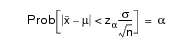
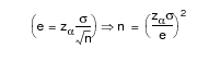
Because  is the estimator for μ, the error is simply the absolute value of the difference between these two values. Then if e is the upper bound on the error with certainty α, the number of required samples n is given by:
Small Sample Confidence Estimates
Note that the above expressions for confidence limits on the mean μ rely on knowledge of the standard deviation  . However, it is not necessarily the case that this quantity is known because the actual distribution of X is not known. If the sample size N is sufficiently large (generally >= 30), the sample variance can be used in place of the true variance to compute confidence intervals.
For cases where variance is unknown and the sample size is small, a method is used that is similar to the one described above, but is based on the T-distribution rather than the normal distribution. The T-distribution resembles the normal distribution in its characteristic "bell curve" shape. However, this distribution is based on the use of the sample variance rather than the assumed or known variance. It is therefore useful for simulation studies where fewer than 30 samples are used to estimate μ, which is actually a frequent case.
As the number of samples become large, the T-distribution begins to approximate the normal distribution. In calculating confidence intervals, the Results Browser uses the sample size 30 as a threshold to begin using the normal distribution. For all sample sets with fewer than 30 values, the T-distribution is used instead. The expressions for confidence limits in this case are similar, except that the true variance  is replaced by the sample variance s², as shown below, and the constant t_α is used rather than z_α to represent areas under the distribution's curve.
Some common values of t_α are provided in the following table. More extensive tables are available in standard statistics textbooks.
Table 137: Common Values of t_α
| confidence level α | t_α, N = 3 | t_α, N = 5 | t_α, N = 10 | t_α, N = 20 |
|---|---|---|---|---|
| 99% | 9.925 | 4.604 | 3.250 | 2.861 |
| 98% | 6.965 | 3.747 | 2.821 | 2.539 |
| 95% | 4.303 | 2.776 | 2.262 | 2.093 |
| 90% | 2.920 | 2.132 | 1.833 | 1.729 |
| 80% | 1.886 | 1.533 | 1.383 | 1.328 |
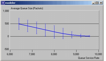
When the Show Confidence Interval operation is applied to a panel, the statistics are shown such that entries aligned on the same abscissa are treated as groups. Each group is collapsed into one entry whose ordinate is the mean of the group. The confidence interval for the mean of each group is calculated using the methods described above and is then displayed as a vertical bar centered at the mean and ending at the upper and lower confidence limits. For entries that are unique at a particular abscissa, no confidence intervals can be calculated. The lack of a confidence bar is indicated by a small circle surrounding the point of interest. This operation offers a choice of five confidence intervals: 80%, 90%, 95%, 98%, 99%. An example of a graph with confidence limits appears below.
Figure 282: Statistic with Confidence Intervals
It is usually possible to control an abscissa variable mapped to the horizontal axis, such that it has the exact same value across multiple simulations. This way, the columns of scalar statistic values are perfectly vertical. However, in some cases, the independent parameter may have some variability due to the fact that it is specified on a stochastic basis. For example, consider a simulation study where performance characteristics of a modeled computer system are to be measured as a function of the job load applied to the system. Suppose in addition, that the job load is specified as a parameter of the simulation, but that the specified value is actually the average job load which controls stochastic job generators within the model. In this case, even with the job load parameter maintained at a constant value, the actual job load would itself vary from simulation to simulation, as random number seeds are changed. Therefore, if the actual job load is taken as the abscissa variable of a scalar versus scalar plot, the groups of points corresponding to a set of identically parameterized simulations will usually not be perfectly vertical.
Because the Show Confidence Interval operation applies only to vertically aligned groups of entries, it is sometimes necessary to eliminate the abscissa coordinate variability of a small group of entries before using this operation. One possible approach that could be adopted in the computer system example, to ensure the alignment of scalar-based entries, is to record the prescribed average job load via the Kernel Procedure op_stat_scalar_write() rather than the actual measured average. This way, the exact same value would be obtained for this parameter, regardless of random number seed.
The Results Browser also computes confidence intervals. Although confidence intervals are computed regardless of the actual content of a panel, the provided result is only meaningful for data sets of a certain nature. In particular, the entries of the panel's statistic(s) must be considered independent samples of a random variable; this determination is left to the user because the Results Browser has no information concerning the source of the statistic data. Under appropriate circumstances, the reported confidence limits for the five confidence levels 80%, 90%, 95%, 98%, and 99% may be used to provide an interval estimate for the mean value of a series of samples contained in a statistic. To display confidence intervals, choose Edit Graph Properties from a Graph pop-up menu and select the Show Confidence Intervals checkbox.