Analysis Data: Statistics
The graphs displayed in analysis panels represent data sets referred to as statistics. Each statistic consists of a sequence of data points called entries. An entry in turn consists of two real numbers, called the entry's abscissa and ordinate.
Table 134: Statistic Content
| entry index | entry abscissa | entry ordinate |
|---|---|---|
| 0 | x0 | y0 |
| 1 | x1 | y1 |
| 2 | x2 | y2 |
| 3 | x3 | y3 |
| 4 | x4 | y4 |
| 5 | x5 | y5 |
| 6 | x6 | y6 |
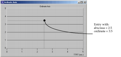
The relationship between the abscissa and ordinate variables is then described by the correspondence established by each of the entries. For a given entry this relationship can usually be read "When the abscissa variable takes on the value x, the ordinate variable takes on the value y", where x and y are the values stored in the entry. In the analysis panel, this entry may be represented by a point located at the intersection of the lines represented by the equations abscissa = x and ordinate = y, as shown in the following figure.
Figure 260: Graphing of an Entry based on Its Abscissa and Ordinate
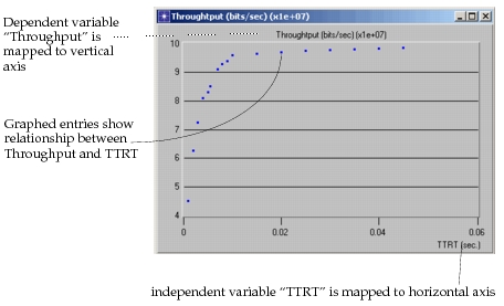
Because each statistic may consist of multiple entries, panels usually contain many points. The resulting graph describes the relationship between the abscissa and the ordinate not only in terms of the dependency at each point, but also by expressing sensitivity of one variable to the other; in other words, graphs can give an indication of the effect that changing one variable has on the other. Usually, if one variable is considered to be varied intentionally, or is treated as a system input parameter, it is called an independent variable and is placed on the horizontal axis. The second variable is called a dependent variable and is mapped to the vertical axis.
Figure 261: Graphing of Dependent Variable vs. Independent Variable
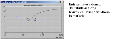
Statistics represented in the Results Browser are intrinsically discrete, even though they might represent relationships between variables of a continuous nature. The spacing of entries within a statistic can be arbitrary, and depends solely on the applications that generate the statistic data (usually a simulation). Irregular spacing of entries on the horizontal axis is a common case because entries are often created as a function of unevenly spaced events in a simulation.
Figure 262: Variable Density of Entry Spacing on Horizontal Axis
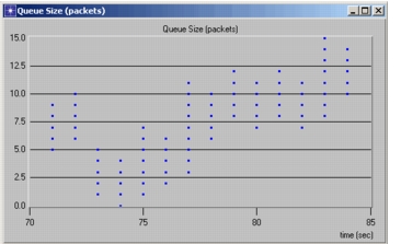
It is possible for a statistic to represent a mapping between abscissa and ordinate variables that is one-to-many. Therefore, a statistic does not necessarily behave as a mathematical function. For instance, multiple ordinate values may occur for an abscissa value as a result of multiple events occurring at the same simulation time and each event generating an additional entry. One such situation is that of a queue that receives many packets at once to be enqueued; as each packet is enqueued, the queue size statistic increases by one, and if the queue is capable of accepting multiple packets at once, multiple values of this statistic will be coincident in time.
Figure 263: Statistic with Multiple Entries Sharing Same Abscissa
Several special entries are defined to represent features of statistics that do not correspond to ordinary numerical data. In some cases, these features are naturally incorporated into certain statistics based on their definitions; in other cases they result from transformations of ordinary statistical data by the operations of the Results Browser.
-
Undefined Value – This type of entry represents a point in the statistic where the system has no knowledge of or cannot compute the ordinate variable, or where it does not make sense to attribute a value to the ordinate variable, based on its definition. For example, the "average queuing delay" statistic for packets in a queue is considered undefined until at least one packet has entered the queue. Similarly, the "signal-to-noise ratio" measured at a receiver for transmissions arriving from a particular source is considered undefined while that source is not active. Undefined values also frequently result from mathematical operations that are not well-defined, such as dividing one zero-valued entry by another, or multiplying an entry with an infinite value by one with a zero-value.
In a graph using the discrete draw style, undefined values are simply omitted from the graph.
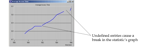
In a graph using the "linear" draw style, the line is suspended until the next defined value. When a defined value is surrounded by undefined values, it appears as a point. The following example shows how undefined value entries appear as gaps in a line graph.
Figure 264: Graph Discontinuities Caused by Undefined Entries
The default graph style changes from linear to discrete if a graph has ten or more disconnected lines or points. (This threshold may be lower for smaller data sets.) You can switch the graph to linear mode in this case, but the line will appear highly fractured.
-
Infinite Value – Like an undefined value entry, this type of entry can arise either from the definition of a statistic or from numerical manipulations performed in the Results Browser. For example, the space available in a queue with unlimited capacity is a statistic that has a permanently infinite value. A common numerical manipulation that generates infinite value entries is dividing a nonzero value entry by one with a zero value. Negative infinite values are differentiated from positive infinite values.
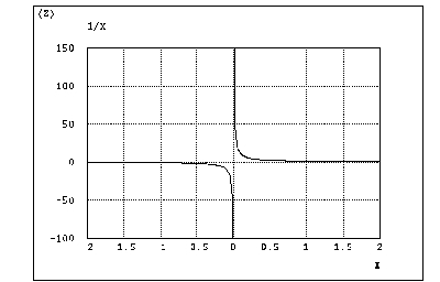
Like an undefined value, an infinite value is omitted from a graph drawn with the discrete style. The linear style distinguishes an infinite value from an undefined value by drawing a line straight up or down (to positive or negative infinity) from the last finite value and then back again to the next finite value. A positive-infinity-to-negative-infinity transition appears as a straight top-to-bottom line. The following panel depicts a statistic for the function
f(x) = 1 / x, containing a negative infinite value followed immediately by a positive infinite value.Figure 265: Example of Statistic Containing Infinite Entries
-
End of statistic – For certain statistics, statistics can be thought of as approximations of continuous mappings between the abscissa and the ordinate variables. Because the tool is limited to a discrete representation, an interpolation method for estimating values between samples is sometimes needed. A particular case of this issue arises at the end of a statistic, when the last entry is recorded at a time that is strictly less than the ending time of a simulation. While no specific ordinate value can be given for the final abscissa, it is useful to know what this abscissa value is, both for plotting purposes, and possibly for users to make their own interpolations. The statistic generation mechanisms of the Simulation Kernel and the Results Browser retain this information by placing a special entry at the final abscissa position of each statistic. This entry is called an end-of-statistic entry.