Event Scheduling and the Event List
A simulation in progress can be viewed both as a generator and a consumer of events. New events are generated by the components of the simulation model to schedule new future activities, based on their underlying behavioral models. Events are consumed as simulation time progresses and specified event times are overtaken.
Discrete event simulations manage events with an event list. The purpose of maintaining an event list is to make sure that all events are executed in the correct time order. Each event has an associated time at which it is specified to occur. The requesting of new events, which requires specification of the simulation time at which they must execute, is called event scheduling. Events are said to be scheduled at particular times. Events may be scheduled for any future time, or for the current time, but never for past times, because the simulation time variable can only progress forward. It is common for new events to be scheduled for the current simulation time because this corresponds to a chain of events that cause each other, using mechanisms that are modeled as having a delay of zero. For example, transfers of packets via packet streams, or values via statistic wires, are both often performed with no delay.
The simulation event list maintains all of the events in time-order so that the next event may be readily determined when the current one has completed execution. The earliest remaining event is referred to as the head of the event list, and the latest event is called the tail. During the execution of each event, new events may be scheduled, including events for the current simulation time. Therefore during execution of an event, the head or tail of the event list may be replaced with a new event. The conceptual structure of the event list is depicted in Figure 67 for a typical set of scheduled events.
Key Concept—Events are managed by the Simulation Kernel in an event list. New events are inserted into the list by the Kernel and by entities within the model. The Kernel extracts the events from the event list and executes them in time-order.
Figure 67: Event List Organization by Execution Time
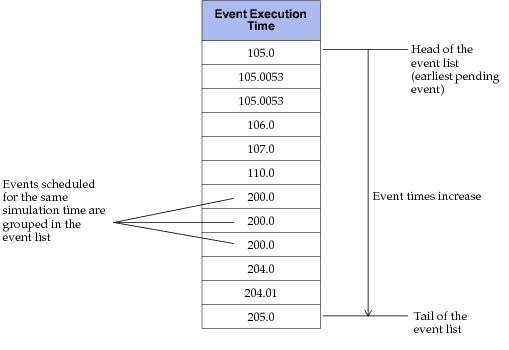
The term “event list” only refers to the conceptual structure of the list. While the events behave as if they are organized in the form of a sequential list, they in fact are stored in proprietary data structures that support very efficient insertion and extraction of events while maintaining the required ordering. The “list-like” abstraction is maintained for all user-visible interfaces to the event storage. In particular, the Ev package of Kernel Procedures, used to scan the event list and query the properties of events, hides the underlying organization from the user.
During a simulation, the event list may continually grow and shrink as new events are scheduled and previously scheduled events are executed or canceled. Each simulation will have its own particular pattern of growth for the event list, depending on the activities that are modeled. Because all future events that are known are scheduled and placed in the event list, a simulation need only continue if the list contains new events to execute. Therefore, if the list becomes empty as a result of executing the last remaining event, a simulation will terminate as that event completes, unless it has in turn scheduled at least one new event. An empty event list will cause a simulation to end regardless of the simulation time elapsed so far.
At the beginning of simulation, the event list must receive at least one event so that execution may begin. The initially scheduled events “bootstrap” the simulation by in turn causing other events. A special type of event called “begin simulation” may be scheduled automatically for processes by enabling the “begsim intrpt” attribute of processor and queue modules within the node domain. Also processor modules automatically choose a time at which to issue their first packet, based on their assigned distributions. These are the types of events that usually appear in the event list when it is examined at the start of simulation.
Key Concept—The event list grows and shrinks as new events are inserted and events are executed over the course of the simulation. At the start of the simulation certain pre-defined events are inserted in the event list to allow execution begin. If the event list becomes empty at any point, the simulation completes.
Event Attributes
So far, events have been presented as abstract items representing simulation activities and having an associated time. However, simulation events have a number of important attributes that provide detailed information about the how the event should be executed. Table 35 lists event attributes.
Note: Depending on the event type, only certain attributes may be relevant.
Key Concept—Each event has a set of event attributes that store information describing it. Some of this information is used by the Simulation Kernel to execute the event. The information may also be used by user-defined logic to process the event in a manner that depends on its characteristics.
Table 35: Event Attributes
| Attribute Name | Attribute Significance / Use |
|---|---|
| time | simulation time at which event should be executed |
| execution ID | unique identifier related to event’s order of execution |
| schedule ID | unique identifier related to event’s order of scheduling |
| module | module (node domain object) where event will occur |
| process | unique process that will receive event |
| type | one of 13 supported classifications of activities |
| code | integer value whose interpretation depends on event’s type; may be user-defined for some events, or represent an arrival port index for others |
| packet | packet whose transmission caused event |
| ICI | Interface Control Information structure coupled to event |
| state_ptr | address of user-defined data block |
| source object ID | Object ID of module of event during which this event was caused. |
The following list provides more information about the event attributes listed in Table 35.
- time – each event has a simulation time at which it is specified to execute. This is a nonnegative double-precision floating-point number that is used to establish an order of execution among the scheduled events. Each event must execute before all events with higher values for the time attribute.
- execution ID – this identifier increases by one for each event as it is executed. Its value is difficult to predict for a given event in the event list, because new events can be inserted, altering the anticipated execution order. The primary use of execution IDs is to refer to events that have already occurred, primarily while analyzing simulations interactively with the Modeler debugger, ODB.
- schedule ID – this identifier follows the order in which new events are generated. Each time a new event is required, it is scheduled by inserting it into the Simulation Kernel’s event list. Because events may be scheduled for any future time (relative to the current simulation time), schedule IDs do not relate in any predictable way to execution IDs.
- module – all simulation events have a designated locality within the node domain which provides a context for their execution. For example, an event may be scheduled to model the arrival of a packet at a particular transmitter; and a statistic change relayed by a statistic wire will cause an event at a particular processor or queue.
- process – because there may be multiple processes within each processor or queue module, certain events must be scheduled while designating the specific process of interest. In particular, self interrupts, used to indicate that an interval has elapsed, must be delivered to a particular process within the surrounding module (specifically, the process that scheduled the interrupt in the first place).
- type – this attribute plays a major role in determining how an event will be processed by the simulation kernel. Depending on an event’s type, the kernel will invoke particular handling mechanisms to execute it. The type of an event is designated when an event is scheduled and is a function of its cause and of the way in which it is intended to be handled. There are 13 types of events, designed to support different types of modeling activities. For instance, an event of type “self” is scheduled by a process and implicitly returns to that same process—it is used for notification of the end of a time-interval; and an event of type “stream” is a result of a packet being sent between two modules. Each event type is described in greater detail in a later part of this section.
- code – certain events may carry an integer code whose value is specified at the time of scheduling. The interpretation of the code varies depending on the type of event. In the case of certain generic events that serve application-specific purposes, this code provides a mechanism for the user to associate additional information with the event and to retrieve in the context where the event is executed, possibly at a later time. For example, a process may maintain many simultaneous interval timers modeled as events of type “self;” it may use the code associated with each event as a method of distinguishing between them. The code attribute is reserved for system use in the case of stream and statistic events where it represents the input stream and input statistic on which packets and new statistic values arrive, respectively.
- packet – several types of events are used to represent activities related to packets such as their arrival at a destination, or the completion of their transmission, for example. The packet attribute simply references the packet of interest for these types of events.
- ICI – interface control information structures (ICIs) are multi-member data items that may be associated with events scheduled by processes. ICIs contain formatted information defined by a user-supplied format. Their purpose is to allow application-specific information, in addition to that intrinsic in a scheduled event, to be communicated to the event’s destination. One common use of this mechanism is to support protocol layers that pass parameters (for example, quality of service, destination, etc.) associated with a transferred packet, to avoid incorporating the parameter values in the packets themselves.
- state_ptr – this event attribute allows a pointer to an arbitrary area of memory to be associated with an event. The content and format of the memory block are user-defined and are not known to the Simulation Kernel. The purpose of this mechanism is to support the transfer of completely general forms of data between the context where the event is scheduled, and the context where it is executed. Currently only “procedure call” events support the use of the state_ptr attribute.
- source object ID – most events are generated by one object for another object, or for themselves. For example, a packet source sends packets to other modules, and schedules events to implement the packet arrivals; and a processor uses scheduling to generate future events for itself. For these cases where an event’s generation can be attributed to a particular module, the source object ID is simply the object ID of that module. In cases where events are scheduled by the Simulation Kernel, such as begin-simulation events, or end-simulation events, the source object ID will have a special value indicating this fact. The exact interpretation of this attribute therefore depends on the event type; for more information, see Event Types.
Event Types
Modeler defines thirteen event types to support a variety of modeling activities. Some event types are used only to represent very specific types of activities, while others are intended for general user-defined purposes. The following table lists the function provided by each event type.
Table 36: Simulation Event Types and Their Applications
| Event Type | Application |
|---|---|
| self | Timers and delayed actions. |
| stream | Communication of packets between modules within the same node. |
| statistic | Asynchronous notification of changes in statistics, semaphores, numeric signals. |
| regular | Automatic, periodic activities such as polling of inputs, transmission of status messages, beginning of bus cycles, etc. |
| failure | Asynchronous notification that a node or link has failed (i.e., condition attribute has become disabled) within the network domain (e.g., allow reconfiguration of routing tables). |
| recovery | Asynchronous notification that a node or link has recovered from failure. |
| begin simulation | Notification of start of simulation, allowing processes to initialize their state. |
| end simulation | Notification of end of simulation, allowing processes to record final information such as scalar statistics, custom reports. |
| access | Generation of a request by one process for another. |
| remote | Communication of commands, requests indications, or other general information between modules, without requiring any physical connections; modules may be in different nodes. |
| procedure call | User-defined purpose requiring a procedure call to occur at some future time. |
| multicast | Simultaneous invocation of all processor and queue modules in entire modeled system. |
| process | Direct invocation of a particular process within a module, rather than the root or other registered process. |
Events can be created by a number of mechanisms that might be driven by the Simulation Kernel or by the logic that is part of user-provided models. The Kernel generally concerns itself with scheduling events that result simply from the configuration of object attributes, such as regular events that occur due to the assignment of the ”intrpt interval” attribute of a processor or queue; another important example is the scheduling of “begin simulation” events for all processors and queues that have the “begsim intrpt” attribute enabled. User-defined processes, on the other hand, are the sources of events relating to general activities such as communication of information, accessing of resources, and handling of alarm conditions, for example. The following table lists the possible ways in which each event type can be generated.
Table 37: Event Generation Mechanisms
| Event Type | Generation Mechanism |
|---|---|
| self | call the KP op_intrpt_schedule_self () |
| stream | forwarding of a packet using any of the KPs op_pk_send...(), or op_pk_deliver...() |
| statistic | updating of a statistic, either automatically by the Kernel or by a call to the KP op_stat_write() |
| regular | automatically provided by the kernel if “intrpt interval” attribute of processor or queue is not disabled |
| failure | automatically provided by kernel to processors and queues that don’t have the “failure intrpts” attribute disabled whenever a node or link’s condition attribute becomes disabled |
| recovery | automatically provided by kernel to processors and queues that don’t have the “recovery intrpts” attribute disabled whenever a node or link’s condition attribute becomes enabled |
| begin simulation | automatically provided by kernel at start of simulations for processors and queues that have the “begsim intrpt” attribute enabled |
| end simulation | automatically provided by kernel at end of simulations for processors and queues that have the “endsim intrpt” attribute enabled |
| access | call to the KP op_strm_access() |
| remote | call to the KP op_intrpt_schedule_remote() or op_intrpt_force_remote() |
| procedure call | call to the KP op_intrpt_schedule_call() |
| multicast | call to the KP op_intrpt_schedule_mcast_global() |
| process | call to the KP op_intrpt_schedule_process() |
Depending upon the type of event, it will make use of certain event attributes described in the previous section. The event type is itself an attribute, but it is not always sufficient to describe the actual work that must be done to execute the event. The appropriate remaining attributes are set when an event is scheduled, and are stored with the event when it is placed in the event list. This information is then available for use in the event’s execution when its simulation time arrives. The following table summarizes the relevant attributes for each type of supported event. Note that standard attributes that have similar interpretation for all event types, such as time, execution ID, schedule ID, module, and type, are not listed in the following table.
Table 38: Significance of Principal Event Attributes
| Event Type | Attribute Significance |
|---|---|
| self | code – integer value with user-defined interpretation; typically used to identify self event among all those scheduled for a given process; accessed with op_ev_code(). ICI – optional, general info. provided when this event is scheduled. source object ID – same as module that is receiving the event. |
| stream | code – index of stream on which packet arrives and can be obtained; accessed via op_ev_strm(). ICI – optional, general info. provided when packet is sent. packet – packet whose reception caused event. source object ID – module that sent the packet, causing the event. |
| statistic | code – index of input connected to statistic wire whose source value has changed; accessed via op_ev_stat(). ICI – optional, general info. provided when statistic is updated. source object ID – module that updated statistic, causing the event |
| regular | source object ID – equal to constant OPC_OBJID_KERNEL. |
| failure | source object ID – object ID of node or link that has failed. |
| recovery | source object ID – object ID of node or link that has recovered. |
| begin simulation | source object ID – equal to constant OPC_OBJID_KERNEL. |
| end simulation | source object ID – equal to constant OPC_OBJID_KERNEL. |
| access | code – index of output stream on which access request is placed. This is the stream on which a packet would be sent to reach the requesting module; value can be obtained with op_ev_strm(). ICI – optional, general info. provided when access request is made. source object ID – object ID of processor or queue that is performing the access. |
| remote | code – integer value with user-defined interpretation; used to relay simple information, such as status values or command codes; accessed with op_ev_code(). ICI – optional, general info. provided when remote event is requested. source object ID – object ID of processor or queue that is requesting the event. |
| procedure call | code – integer value with user-defined interpretation; used to relay simple information, such as status values or command codes; accessed with op_ev_code(). ICI – optional, general info. provided when procedure call is requested. source object ID – object ID of processor or queue that is requesting the procedure call. state_ptr – optional pointer to area of user-allocated memory that has user-defined content; allows passing of arbitrary state to called procedure (appears as one of the procedure’s arguments). |
| multicast | code – integer value with user-defined interpretation; used to relay simple information, such as status values or command codes; accessed with op_ev_code(). ICI – optional, general info. provided when multicast event is requested. |
| process | code – integer value with user-defined interpretation; used to relay simple information, such as status values or command codes; accessed with op_ev_code(). ICI – optional, general info. provided when process event is requested. process – handle of process that is invoked when the event is executed.; used by kernel to invoke the process. |
Event Processing
There are certain actions that are commonly performed when processing each type of event. These actions typically acquire information that accompanies the event to set up for application-specific execution actions and decision-making. These common actions are presented in this section, on a per event type basis, to familiarize the developer with the type of logic that is typically found in process models.
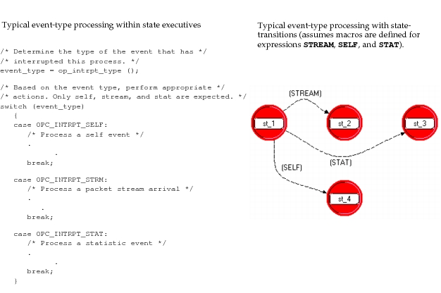
Most processes, especially those that manage complex interactions, must be capable of handling the arrival of several different types of events while located in each state. Therefore, one of the basic actions that is performed as part of the logic on state executives and/or in transition conditions is to determine the type of event that has occurred. The Kernel Procedure (KP) used for this purpose is called op_intrpt_type() and its use is illustrated in the following example. The event type is just one of the event attributes that a process’ logic might analyze. In general, attributes of an event can be obtained using KPs from the Event (or Ev) Package of the Simulation Kernel. Certain KPs in the Interrupt (or Intrpt) package can also be used. The difference between Ev KPs and Intrpt KPs is that Ev KPs can be applied to any event, including future events that are still stored in the Event List. Intrpt KPs on the other hand, such as op_intrpt_type(), implicitly refer to the currently executing event.
Key Concept—When a process model handles an event, it usually needs to analyze certain attributes of the event, such as the event’s type, to determine the actions that it will take. The attributes can be obtained using KPs of the Ev and Intrpt packages.
Figure 68: Common Process Model Forms for Processing Based on Event Type
-
Self – for processes that may have multiple events of this type pending at a time (e.g., a protocol that maintains multiple timers), the event code is usually of interest. How it is used is determined entirely by the process’ logic. Typically, the code is an identifier for an object maintained by the process, such as a particular timer, a counter to be modified, or a packet to be retransmitted. Figure 69 shows the retrieval of the event code and its use.
Figure 69: Typical Processing of an Event of Type “Self”
/* The event is of type 'self': obtain the event code */ /* representing the timer that has expired. */ timer_index = op_intrpt_code (); /* Depending on which timer has expired, increment the */ /* lateness counter, or make a retransmission */ if (timer_index == TIMER_ROTATION) lateness_counter++; else retransmit_last_packet(); -
Stream – when a packet arrives at a processor or queue, causing a stream interrupt, the Simulation Kernel places the packet in the input stream’s FIFO queue. The process may choose to leave it there, or to accept it. Because a process can maintain several input streams (i.e., it may be connected to several sources of packets), it may need to determine the input stream via which the new packet has arrived. This determination, and the logic needed to obtain the new packet, are illustrated in the Proto‑C fragment in the following figure.
Figure 70: Typical Processing of an Event of Type “Stream”
/* The event is of type 'stream': obtain the index of */ /* the input stream on which the packet has arrived. */ input_stream_index = op_intrpt_strm (); /* If the packet has arrived on the stream coming from */ /* the network, accept it now. */ if (input_stream_index == STREAM_NETWORK) packet = op_pk_get (STREAM_NETWORK); -
Statistic – when a change occurs in a statistic that is the source of a statistic wire, this may generate an event for the statistic wire’s destination processor/queue, depending on the nature of the change and the configuration of the statistic wire object. Because the processor/queue can maintain multiple statistic inputs, the first step that is taken is usually to determine which input is associated with the event. A typical Proto‑C processing sequence that reacts to a statistic event is shown in the following figure.
Figure 71: Typical Processing of an Event of Type “Statistic”
/* The event is of type 'statistic': obtain the index of */ /* the input statistic connected to the active statistic. */ /* wire. */ input_stat_index = op_intrpt_stat (); /* If the changed statistic represents the size of the */ /* packet queue, obtain the new value to test for a */ /* critical condition. */ if (input_stat_index == STAT_QUEUE_SIZE) { current_q_size = op_stat_local_read (STAT_QUEUE_SIZE); if (current_q_size >= CRITICAL_LEVEL) { start_alarm (); } } -
Regular – this type of event is provided by the system at periodic intervals. There are no attributes of interest associated with regular events. The significance of the event varies from application to application, and so no typical example is provided here.
-
Failure and Recovery – the system automatically provides these types of events to appropriately configured processors and queues when the condition attributes of nodes or links are changed to the values “disabled” and “enabled”, respectively. Typically, the processes that are affected need to determine the identity of the node or link that caused the event to occur. Figure 72 shows how this is accomplished.
Figure 72: Typical Processing of Event of Type “Failure” and “Recovery”
/* Determine if this is a failure or a recovery */ event_type = op_intrpt_type (); if (event_type == OPC_INTRPT_FAIL) status = DOWN; else status = UP; /* Determine the object ID of */ /* node or link whose status has been affected. */ object_id = op_intrpt_source (); /* Determine if the object is a node or a link. */ object_type = op_id_to_type (object_id); if (object_type == OPC_OBJTYPE_NDFIX) { /* Reconfigure routes as a result of node changes. */ routes_reconfig_node (object_id, status); } /* Otherwise, reconfigure to reflect link change. */ else routes_reconfig_link (object_id, status); -
Begin simulation – this type of event is automatically provided by the kernel to each processor or queue that has the “begsim intrpt” attribute set to the value “enabled”. There are no special event attributes associated with begin-simulation events. In fact, many processes simply assume that their first event will be of this type, and do not even bother to determine the event type in their initial logic. This type of event is usually needed to allow processes to initialize their state variables. Because process state memory can be defined very generally by the user, initialization may involve a wide variety of actions. A typical operation performed at initialization involves “learning” values that have been assigned to process attributes. This is illustrated in Figure 73.
Figure 73: Typical Processing of an Event of Type “Begin Simulation”
/** This is the first invocation of this process. **/ /** Setup initial values of state variables. **/ /* Obtain the object ID of the processor in which this */ /* process is running. */ this_proc_id = op_id_self (); /* Obtain the values of the service rate and maximum */ /* packet size attributes of the processor and store */ /* these values in corresponding state variables. */ op_ima_obj_attr_get (this_proc_id, "service rate", &service_rate); op_ima_obj_attr_get (this_proc_id, "max packet size", &max_packet_size); /* Initialize other state variables. */ num_packets_processed = 0; busy = 0; -
End simulation – when a simulation reaches termination, regardless of the reason, all processors and queues that have the “endsim intrpt” attribute set to the value “enabled” receive an event of this type. There are no special event attributes that provide additional information about the resulting invocation, and the processing that takes place can vary widely from application to application. Typically end-of-simulation tasks have to do with customized reporting based on information accumulated during an entire simulation run. The Proto‑C fragment in Figure 74 provides an example of such processing.
Figure 74: Typical Processing of an Event of Type “End Simulation”
/* The simulation has completed, except for end-simulation */ /* events. Perform final actions for this process. */ /* Compute final average performance statistics. */ total_time = op_sim_time (); average_throughput = num_packets_processed / total_time; average_utilization = total_busy_time / total_time; average_delay = total_delay / num_packets_processed; /* Write these values out as scalar statistics. */ op_stat_scalar_write ("average throughput", average_throughput); op_stat_scalar_write ("average utilization", average_utilization); op_stat_scalar_write ("average delay", average_delay); -
Access – access requests are issued by a module that is the destination of a packet stream. The source module receives an event and can determine which stream (an output stream from its perspective) was used to convey the request. This type of event usually (but not necessarily) indicates a request to have a packet forwarded by the source module on the specified stream. The Proto‑C fragment in Figure 75 is an example of how a process might respond to the receipt of an event of type access.
Figure 75: Typical Processing of an Event of Type “Access”
/* A request to forward a packet has been received. */ /* Determine which outgoing packet stream leads to the */ /* requesting module. */ out_stream = op_intrpt_strm (); /* If there are packets available in this module’s queue, */ /* remove the highest priority one and send it. */ if (op_subq_empty (MAIN_SUBQ) == OPC_FALSE) { packet = op_subq_pk_remove (MAIN_SUBQ, OPC_QPOS_PRIO); op_pk_send (packet, out_stream); } -
Remote – remote events are generated by one processor or queue for another processor or queue. The same attributes are associated with these events as are with events of type “self”. However, because remote events can be communicated to other modules, and particularly, to modules that are not physically connected, they are often used to represent commands, requests, or indications. Figure 76 shows a Proto‑C specification that implements the receiving end of an interface based on remote events. In this example, the event code is not used because the more general ICI can superset the code’s functionality.
Figure 76: Typical Processing of an Event of Type “Remote”
/* A remote event has been received; this represents a */ /* command from one of the remote nodes. */ /* Obtain the ICI associated with the event: it contains */ /* all the parameters of the command. */ ici = op_intrpt_ici (); /* Obtain the command type parameter. */ op_ici_attr_get (ici, "command type", &command_type); if (command_type == COMMAND_FLOW_OPEN) { /* Open a new buffer for a new flow of data. */ /* Obtain relevant parameters of the command. */ op_ici_attr_get (ici, "peak rate", &peak_rate); op_ici_attr_get (ici, "flow src", &flow_src); op_ici_attr_get (ici, "flow dst", &flow_dst); /* Create the new flow. */ create_new_flow (flow_src, flow_dst, peak_rate); } else if (command_type == COMMAND_FLOW_RESIZE) • • • -
Procedure call – this is a special type of event that provides a very general, “open” interface for integrating external software into a discrete event simulation. The event results in the invocation of a procedure with a predetermined argument list. The context of the invocation is still the module where the event was originally scheduled. Several event attributes might apply, as explained earlier in this section and illustrated in the sample C language procedure definition in Figure 77.
Figure 77: Typical Processing of an Event of Type “Procedure Call”
void discard_enqueued_packet (char* state_ptr; int code) { int subq_index; Packet* pk; /* This procedure is invoked as a scheduled event in */ /* order to remove a particular packet from a subqueue.*/ /* the subqueue is specified by the event code and the */ /* packet address is given by the 'state_ptr' arg. */ subq_index = code; pk = (Packet*) state_ptr; /* Find the packet in the subqueue, remove, destroy it. */ subq_size = op_subq_stat (subq_index, OPC_STAT_PKSIZE); for (i = 0; i < subq_size; i++) { if (op_subq_access (subq_index, i) == pk) { op_subq_pk_remove (subq_index, i); op_pk_destroy (pkptr); break; } } } -
Multicast – these events are provided to all processors and queues in the entire system model. They are typically used to support synchronized operations such as modeling a complete resetting of state throughout the system; or a delineation of “epochs” in the simulation, where objects are forced to reconfigure before simulation can continue. The application of the interrupt is user-defined and supports the use of an ICI and an event code. Figure 78 shows a possible Proto‑C specification for responding to a multicast event.
Figure 78: Typical Processing of an Event of Type “Multicast”
/* A multicast event has occurred; examine the code to */ /* determine what behavior is expected. */ event_code = op_intrpt_code (); if (event_code == GLOBAL_RESET) { /* this event represents a globalized resetting */ /* of all state throughout the system. This process */ /* need only reset its private state memory. */ /* eliminate packets in all the subqueues. */ op_q_flush (); /* reset the state variables kept for estimating */ /* timer values. */ total_packets = 0; total_delay = 0.0; round_trip_time = INTITAL_RTT; } -
Process – most event types are directed at modules in general, but process events are intended to invoke a particular process within a processor or queue’s context. Often a process event is scheduled by one process for another in its same processor or queue (e.g., its parent or child process). This can be viewed as a deferred invocation, providing an alternative to the immediate invocation that is commonly used between processes. Process interrupts make use of the same event attributes as self interrupts; an example of Proto‑C code that responds to a “process” event appears in Figure 79.
Figure 79: Typical Processing of an Event of Type “Process”
/* A process event has occurred and has caused */
/* this process to be invoked. */

/* Determine the reason for invocation, which is provided */
/* as the event code. */
invoke_code = op_intrpt_code ();

/* At this point, this process can be invoked for */
/* two reasons: to begin transmissions or to reset */
/* the connection that it manages. */
if (invoke_code == XMIT_START)
	send_packets ();
else reset_connection ();
Interrupts
In addition to events, Modeler defines the related notion of an interrupt. Events may be viewed as requests for activities to occur at particular times. In contrast, interrupts are defined as the actual invocations that result from events being executed by the Simulation Kernel. In other words, events that are in the event list become interrupts only when they are delivered to the modules that they are destined for. Interrupts never actually reside in the event list.
Interrupt Attributes
Interrupts have the same attributes as the events that generate them. In particular, interrupt types use the same names (stream, statistic, self, and so on). Because an interrupt is the manifestation of an event that is executing, its attributes can be accessed by obtaining a handle for the current event and applying KPs of the Ev package, such as op_ev_code(), op_ev_ici(), and op_ev_src_id(). However, because these operations are common with regard to the current event (that is, a process tends to need information about its current invocation more often than about future ones), a number of KPs in the Intrpt package operate implicitly on the current event. The following table summarizes the KPs that provide access to interrupt attributes; see Chapter 11 “Interrupt Package” on page 1 for more information about these KPs.
Table 39: Kernel Procedures that Access Interrupt Attributes
| KP | Attribute |
|---|---|
| op_intrpt_type() | Type |
| op_intrpt_code() | Code |
| op_intrpt_strm() | Input stream of packet arrival |
| op_intrpt_stat() | Input statistic |
| op_intrpt_source() | Source object ID |
| op_intrpt_ici() | ICI (interface control information) |
Key Concept—An interrupt occurs when an event reaches the earliest position in the event list and becomes executed. The interrupt is delivered to the event’s destination object and has most of the same attributes as the event.
Interrupt Suppression
Certain events may be executed and still not result in the generation of an interrupt. This may happen as a result of various suppression mechanisms that apply to some events at the time when they are executed.
The most common form of interrupt suppression is established by a process to limit the arrival of unwanted interrupts, either during a particular interval, or for an indefinite period. The process can accomplish this by calling the KP op_intrpt_disable(), as necessary to affect various combinations of interrupts. Each call specifies a type of interrupt, optionally combined with an interrupt code.
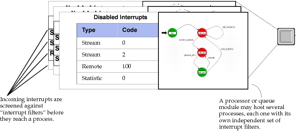
The effect of calling op_intrpt_disable() is cumulative from call to call, meaning that several sequential calls may be used to disable multiple types of interrupts. Conceptually, one may view the process as maintaining a list of “interrupt filters” on a per process basis (not on a per processor or queue basis). Each interrupt filter, as long as it is present, prevents a particular interrupt type and code from reaching the process, as shown in the following figure.
Figure 80: Suppression of Interrupts on a Per-Process Basis
Typically, the interrupt disabling mechanism is used when a process enters a phase during which certain interrupts cannot be processed, due to some sort of a busy condition. For example, a transmission management subsystem implemented by a processor may be unable to handle more than one transmission request at a time; rather than having to interrupt its processing of a packet transmission to deal with new asynchronous packet arrivals, it may choose simply to disable all stream interrupts until it has completed the one on which it is busy working. When the current transmission has completed, the packets that arrived in the interim, but failed to cause interrupts, will be queued in the processor’s input stream(s).
Most disabled interrupts do not automatically queue to provide an indication that they occurred. Packets causing stream interrupts do queue during the time that they are disabled because each packet contains unique information and it is usually desirable to have no “gaps” in packet sequences. On the other hand, information lost due to suppression of statistic interrupts, remote interrupts, or other types, cannot be recovered by a process that had disabled them.
The effect of interrupt-disabling is reversible by several mechanisms. One common form of reversal is built-in to the disabling request itself; calls to op_intrpt_disable() support the specification of a parameter called next that renders the interrupt-suppression valid only for one occurrence of the interrupt; interrupt controls specified this way are removed immediately after they have served to prevent the delivery of one interrupt. When suppressing interrupts for a period of time, or until some logical condition has been reached, a process usually re-enables the interrupts via the KPs op_intrpt_enable() or op_intrpt_enable_all(). The former KP is used to enable a specific combination of interrupt type and interrupt code, while the latter KP removes all interrupt controls for the process (i.e., this KP returns the process to its default state where no interrupts are suppressed). See “Interrupt Package” on page 1 for more information about the applicability and usage of these KPs.
Key Concept—A process may prevent certain events from being delivered to it as interrupts when it knows that it can safely ignore them. This is done to simplify the process model and to improve simulation speed. Interrupts may be disabled and re-enabled based on certain attributes using the KPs of the Intrpt package.
Modeling Actions that Involve Delays
Whether models are designed with the objective of measuring performance or analyzing behavior, it is often important to accurately model delays associated with key actions to obtain representative results. Common performance metrics, such as resource utilization (of links or processors, for example) and end-to-end delay of messages, are largely a function of various delays incurred by messages, transactions, or jobs, depending on the application. Also, metrics such as queue sizes and throughputs are indirectly dependent on processing delays because the delays incurred at particular locations in a system may create “bottlenecks”. Behavior of the system is also tied to delays, because timing of communications between components may critically affect the order in which actions are taken, and even which ones are taken. For example, delays of acknowledgments expected by a flow control and error recovery subsystem may cause an unusually high number of retransmissions, or may cause the system to reach a deadlock state, depending on its specific design. The behavior that is actually observed always depends on how the various subsystems are defined, and the interaction between subsystems is often affected by delays in communication or processing.
Modeler supports techniques for incorporating delays into system models. The appropriateness of the various methods depend to a large extent on the type of action with which a delay is associated, and at what point in the system the delay is occurring. The following is a list of sample actions that commonly require delay modeling:
- Computations required to complete a task or sub-task – computations of many different types are generally necessary to implement decision-making subsystems; the computations that are required in the actual subsystem (not the modeled one) should be analyzed to determine the delays they require. If these time intervals are significant, the developer should consider including them in the model. Some typical tasks requiring delays when modeling network protocols are: evaluating intactness of received data (i.e., calculation of checksums); compression/decompression of transmitted/received data; construction of a packet given some general data and “header” information (e.g., destination address, service class, etc.); decoding and demultiplexing of a properly received packet. For general system modeling, tasks will depend heavily on the application and may fall in a broad range, from executing signal-processing algorithms to interpreting telemetry data, or refreshing a radar display.
- Transmission and propagation between two components – depending on the physical relationship between components, or the mechanism by which they communicate, delay can be a significant factor in their interaction. In some cases, communication between two components may not rely on a physical connection, but instead be implemented in an abstract form, such as when a procedure call is executed within a software program. Communication delay between two components that are physically connected by some sort of channel can usually be attributed to propagation delay and transmission delay; the former is the time required for information to travel between the two components, and the latter is time required to insert the information into the communication channel. In some cases, one or the other, or both may be ignored. For more abstract forms of communication, delays may represent the inherent limitations of the information transfer mechanism; in the case of a procedure call, the primary delay may result from the execution of CPU instructions required to setup arguments and transfer control to a new location in a program, as well as the possible loading of new program instructions from disk (i.e., swapping of a program segment).
- Reading/writing information to/from storage devices – most systems maintain state information, either as their primary function, or in support of other activities. Certain events provoke changes in, or make use of this information, or combinations of both. The information of interest may be maintained in one or more devices depending on the system’s storage architecture; these devices are typically general semiconductor memory, cache or display memory, microprocessor registers, magnetic or optical disk, magnetic tape, or in a more abstract sense, even remote databases accessed via a network. Depending on which devices are used and the volumes of data that are accessed, read and write operations may introduce significant delays into the operations they support.
- Reaction to a major event, requiring reconfiguration – certain events may require a subsystem to reconfigure to adapt to a modified operating environment. Such situations often occur in modeling efforts that study a system’s robustness to failure of one or more components. The failure of a key component may trigger significant activity, such as recomputation of routes to bypass the lost resource, or even complete initialization of other components’ state. The recovery of such a component may trigger similar activities as the system attempts to maximize its use of available resources. Because robustness studies frequently include as a goal the determination of the time required to adapt to a major system alteration, the delays encountered in each involved action may be significant aspects of the system model.
The examples above merely illustrate the need to model certain delays to develop accurate simulations that are capable of reliably forecasting system performance and behavior; there are, of course, many other situations where the activities that are modeled require incorporation of delay effects. These examples do support a number of important points however, with regard to modeling delays:
- Not all delays need to be modeled – Certain delays are insignificant in relation to others. Yet these delays may require as much modeling effort as those that tangibly affect the system’s performance or behavior. For example, obtaining information such as the number of retransmission attempts made by a protocol, may involve a simple memory register access, and therefore incur only a minute delay; on the other hand, performing an address mapping may rely on reading a file from disk, which requires a much greater delay. It would therefore probably be wise to model the address mapping operation’s delay rather than the variable access; avoiding the additional complexity of modeling the delay of very fast operations may impact the model’s overall accuracy in a negligible manner. This is particularly true if a slow and a fast operation happen together or if the slower operation occurs with greater frequency. It is worth noting, however, that even a very fast operation may have a noticeable cumulative effect if it happens very often.
- Delay values may be difficult to obtain – Many delays are not precisely known at the time of model development. In some cases the required delay values are the result of complex interactions that are beyond the scope of the modeled system. For example, disk access delays may be the result of contention for a computer bus by devices that are not even part of the system model; or the disk itself may be busy on behalf of other processes. Such variable delays could be modeled as random variables, but probability distributions must then be specified. One possible method for obtaining required delay values is to do benchmarking on an actual component if it exists, or to obtain estimates from the component’s manufacturer. If a component is hypothetical, the modeler must simply provide educated estimates for the delays, or treat them as system parameters that can be used as the basis for parametric evaluation (that is, as different delay values are considered, what is the effect on system performance?). In all cases, it should be noted that Modeler has no prior knowledge of the components being modeled and is therefore not cognizant of the correct delay values; nor does it realize which actions are associated with significant delays, and which ones represent negligible delays. It is the responsibility of the model developer to supply these basic values; in turn, it is the role of the simulation to emulate the specified delays and to therefore implicitly produce representative behavior and performance with correct aggregate delays as well as other phenomena.
- Certain actions of the real system may be modeled exclusively by their delay – In many cases, the operations of an actual system will not be modeled in complete detail, either for simplification, or because they would not impact the simulation’s operation. For example, the receipt of a packet by a data-link layer protocol may involve as a first step, the verification of data integrity by means of a checksum computation; the protocol may then proceed to obtain values of various fields in the packet to do its data-link functions. A typical model of this protocol would not do the checksum computation, because the mechanics of this computation are not directly relevant to the model’s emulation of the actual protocol’s behavior. However, aspects of the checksum operation that may matter for the model’s accuracy are the time required by the calculation, and possibly its result (i.e., determination of the data’s validity or corruption). Therefore, it is sometimes important to incorporate the delay effects of operations even though they are not explicitly represented for any other modeling purpose. As mentioned earlier, the converse of this principal is also true—namely that certain operations that are explicitly modeled in terms of their mechanics or behavior need not necessarily be modeled in terms of the delay they introduce. In particular, note that operations that are pure artifacts of simulation, such as calculation of statistics for reporting purposes, should generally be modeled as having no delay.
Key Concept—The modeler must decide which actions of a system should be modeled. In general, those delays that affect the desired system statistics in a measurable way should be accounted for. In certain cases, delays may be the only aspect of a system action that is actually modeled; also, some actions may be modeled as having no delay.
Techniques for Representing Delays
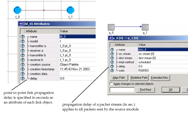
The simplest types of delays in models are associated with the transfer of information over links between nodes in a network, or between modules within a node. The types of delays encountered in these situations are propagation delay and transmission delay. In almost all models, both types of delays are set via the attributes of the corresponding link or connection object. In the case of link models, actual delay values are computed based on link properties by the underlying link models, known as transceiver pipeline stages. See Chapter 9 “Communication Mechanisms” on page 331 for more information about link models.
Figure 81: Propagation Delay Specified as Attributes of Links and Connections
This section concentrates on the delays inherent in the operations performed by process models, because these typically require more careful implementation. These delays can be implemented via a variety of techniques. The key difficulty in modeling finite-time operations is that no single event can occupy a simulation time-span greater than zero. Therefore more than one event is required to represent such an operation. There are two general forms of event-scheduling used to represent a finite-time operation. The first form, referred to as external delay modeling, places the burden of delayed action on the Kernel; the second form, referred to as internal delay modeling, relies on the component performing the action to manage the timing as well as the execution. Both techniques use two events to implement a finite-time operation; one event starts the operation, and the second marks its completion.
External delay modeling provides the simplest interface to the model developer. It is applicable whenever all information required to specify an action is available when it begins, and the component performing the action requires no notification that the action has completed. In other words, the effects of completing the action are entirely external to the component performing it. A common example of external delay modeling makes use of the Kernel Procedure op_pk_send_delayed() to send a packet out of a module via a packet stream. This procedure allows the specification of a delay time for which the Simulation Kernel should hold the packet prior to forwarding it. The specified delay can be used, for instance, to represent processing time or transmission time associated with the sending of the packet. From the perspective of the destination module all delays are correctly modeled, because the packet arrives at the correct time. The following diagram shows a packet transmission/reception sequence for external delay modeling of a fixed processing delay.
Figure 82: External Delay Modeling: Processing Time Incorporated into Packet Forwarding
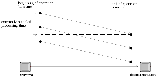
The preceding example highlights one of the potential pitfalls of external delay modeling. Note that the processing time is greater than the time separating consecutive transmissions. This modeling is correct if the source processor is capable of simultaneously processing two packets; however, if instead the processor can only manage the processing and transmission of one packet at a time, then the model is inaccurate, because it allows the second packet’s processing and transmission to begin before the first one’s processing has ended. The intersecting horizontal and diagonal lines in the diagram highlight this error.
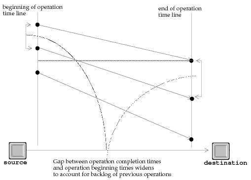
One possible solution to the simultaneous processing problem presented by the external delay modeling technique involves accounting for the backlogged processing time within the component performing the action. To correct the error in the example above, the processor called “source” would incorporate additional delay into the forwarding of the second packet to account for the time that this packet would normally have waited while processing of the first packet completed. Note that this even further increases the amount of time that the third packet must be delayed. The best way to implement this system correctly while still using external delay modeling is to use a variable in the source process to represent the next available processing and transmission time, and to adjust this variable as each transmission occurs. A Proto‑C fragment that could be used to implement this technique is shown below, as well as the resulting packet transmission/reception sequence.
Figure 83: Example Implementation of External Delay Modeling with Single-Threaded Processing
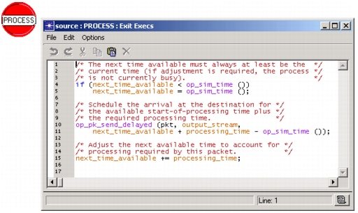
Figure 84: Start/End Timeline for External Delay Modeling with Single-Threaded Processing
As a final note on external delay modeling, the following table lists the Kernel Procedures, similar to op_pk_send_delayed(), that support this technique.
Table 40: Kernel Procedures Supporting External Delay Modeling
- op_pk_deliver_delayed()
- op_pk_send_delayed()
- op_intrpt_schedule_remote()
- op_intrpt_schedule_call()
- op_intrpt_schedule_process()
Internal delay modeling is a natural implementation of processing delay because it is performed entirely in the location where the operation itself takes place. The technique consists of recording state information that reflects that an operation has begun, and of simultaneously starting a mechanism that will interrupt the process when the operation ends. If the duration of the operation is known when it begins, then this mechanism is typically a self-interrupt scheduled via the Kernel Procedure op_intrpt_schedule_self(). The recorded state information is typically used to prevent redundant use of the processing resource and/or to complete the operation when the later interrupt is received. In many cases, some sort of “busy” variable is used to account for the fact that a process is already engaged in completing a task.
Internal delay modeling is the only recommended method when the delay of interest is associated with a local operation that does not result in some type of communication with other modules. It is a commonly used technique, because many processing delays are associated with entirely local actions. For example, a processor may receive a packet that contains a routing topology update, and require a certain processing time to reconfigure its routing table; or a queue may receive a command to flush its contents and prevent further actions until this operation has completed. The following fragment of a Proto‑C model shows the implementation of internal delay modeling for such a queue. In this case the process does not leave the FLUSH state until the flushing operation is complete; all interrupts that occur in the interim are ignored, so no special state variables are needed to keep track of the fact that the process is busy performing this operation. The condition FLUSH_OPERATION_COMPLETE specifies both the interrupt type and code must correspond to the self interrupt requested earlier in the FLUSH state to allow the process to return to the IDLE state.
Figure 85: Implementation of Internal Delay Modeling for a Simple Process
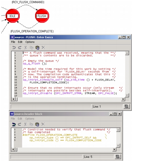
Note that a generally equivalent form of internal delay modeling is possible whereby the operation whose delay is modeled is performed at the end of the waiting period rather than at the beginning, as in the example above. This distinction may be important in cases where the operation results in a change in the system’s state and the timing of such a change is relevant to the model’s behavior (e.g., the operation involves destroying a packet whose contents may still be accessed before completion).
In addition to being used for local operations, internal delay modeling is used whenever any of the following conditions are met:
- The process that is performing the operation does not have knowledge of the delay interval at the time that it begins the operation – This lack of information prevents the process from being able to specify to the Simulation Kernel at what time it should complete the operation, which is required for external delay modeling. Typically, these types of situations arise when a process depends on an externally generated condition to complete a local operation (for example, a statistic interrupt indicating that an external resource is available).
- The process supports any type of preemption that would alter the delay time midway through the operation – For instance, consider a queue whose task it is to forward packets in order of priority and that can suspend service of a packet to accord precedence to another one of higher priority; it would be incorrect for the queue’s algorithm to use the external delay technique and to forward packets at any time before their service intervals completed, because anticipated delays may change due to the subsequent receipt of higher priority packets.
- The operation may affect state information that is not yet available or depend on state information that may change – For example, a process that receives commands, processes them and issues messages based on the command contents might normally be able use external delay modeling to represent the processing time for these commands; however, if in addition, the process may be asynchronously reconfigured by a management process in such a way that the processing times are modified, then the external delay modeling technique breaks down, because it schedules operations to complete at erroneous times (times that would have been valid if the process had not been reconfigured).
If, in a given modeling problem, both internal and external delay modeling are applicable, then the model developer should consider the following facts to decide on the nature of the implementation: (1) external delay modeling provides a simpler interface to the developer, allowing the delay to be fully specified in one place, whereas internal delay modeling may require several states of a process model to be knowledgeable about the operation’s completion event; (2) external delay modeling generates one less event per completed operation than internal delay modeling, which may result in simulation performance improvements; (3) external delay modeling may result in a large number of operations being represented in the event list at the same time, which in extreme cases may result in a simulation performance loss; (4) internal delay modeling is always possible and is therefore more extensible than external delay modeling, as a change in the way delay is computed is less likely to cause a significant change in implementation.
Key Concept—Two general techniques are used to model delays associated with actions: Internal and External delay modeling. External delay modeling schedules the result of an action to take place after the delay elapses. Internal delay modeling schedules an event to mark the end of the delay and during that event, the result of the action is implemented, which may require an additional event.
Event Cancellation
The Simulation Kernel provides a number of interfaces that support processes scheduling future activities for themselves or for other processes. The discrete points of interest in a given activity are represented by interrupts that result from events being scheduled. State information may be associated with the interrupts so that when they actually occur, this information may be retrieved to distinguish them from one another. Interrupts are scheduled to model a number of system features, including processing delay, timer expirations, propagation and transmission delay, resource availability, polling of resources, traffic generation, etc. Earlier parts of this section provide more background on these types of applications and how they may be implemented.
All event-scheduling interfaces are provided by the Simulation Kernel in the form of Kernel Procedures (KPs). Many of these procedures return a special value called an event handle. An event handle (also referred to as an Evhandle because this is their datatype for purposes of declaration) is actually a data structure whose purpose is to retain access to the event that has been requested. A list of the KPs that provide event handles as return values appears below.
Table 41: Kernel Procedures that Schedule Events and Return Event Handles
- op_intrpt_schedule_call()
- op_intrpt_schedule_mcast_global()
- op_intrpt_schedule_process()
- op_intrpt_schedule_remote()
- op_intrpt_schedule_self()
- op_pk_deliver()
- op_pk_deliver_delayed()
- op_pk_send()
- op_pk_send_delayed()
The Simulation Kernel provides an entire package of KPs, called Ev, that operate on event handles. Many of these KPs are concerned with determining attributes of an event or using an event to find other events in the event list. However, the primary application of event handles is the cancellation of scheduled events, using the KP op_ev_cancel().
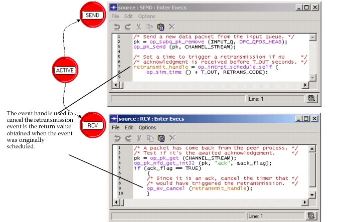
Events that are scheduled may be canceled at any time prior to their execution. Cancellation is even possible during previous events that occur at the same simulation time that the event of interest is scheduled for. Events are canceled for various reasons depending on the application. The general cause of an event cancellation is that an anticipated action is no longer needed or would be inefficient. The most common use of op_ev_cancel() is to revoke the events that mark the expiration of timers; usually these events are scheduled via the KP op_intrpt_schedule_self(). The following Proto‑C model shows the application of this technique to a typical situation where the timer is used to trigger the retransmission of a packet in absence of an acknowledgment from a peer process.
Figure 86: Canceling an Event That Represents a Retransmission Timer
Note: When an event of type “stream” is canceled, the associated packet is automatically destroyed by the Simulation Kernel.
Key Concept—When an event is scheduled, an event handle can be obtained. If the event handle is preserved, it may later be used to cancel the event using the KP op_ev_cancel(). Certain Ev package KPs also provide other ways of obtaining event handles. Events may be canceled at any time prior to their execution.
Interrupt Methods
The Simulation Kernel provides several options with regard to the timing of interrupt deliveries to processes. These options are controlled either via the KPs used to schedule the events of interest, or via the attributes of objects used to facilitate the interrupt. The two broad classes of events are called scheduled and forced.
Scheduled events are the most commonly used form, and are the basis of most of the examples that appear in this section. As their name implies, scheduled events rely on an event scheduling mechanism whereby they are inserted into an event list from which they are extracted in order of their designated simulation time. As explained earlier, an event in progress may schedule events for the same exact simulation time (i.e., the current time). However, these events may not be considered for execution until the current event has completed; instead they are simply inserted into the event list, and when the current event has completed all of its actions, the highest priority event scheduled for the same time is serviced.
Forced events provide an alternative to the deferral of execution that is inherent in event-scheduling, by interrupting the receiving module immediately. This behavior is useful when the interrupt source must obtain some type of result or service from the interrupt destination before continuing its execution. A common example of this type of interaction is used to support extraction of packets from what are referred to as passive queue models. A passive queue waits to be accessed by an externally-generated interrupt before forwarding packets; it accepts packets that are sent to it by its upstream neighbors and enqueues them, but never autonomously forward packets to its downstream neighbors. The externally-generated interrupt is usually an access interrupt resulting from a call by a downstream process to the KP op_strm_access(). This KP generates a forced interrupt for a process in the queue, which forwards a packet according to its own internal rules. The downstream process, which called op_strm_access() to obtain a packet, is blocked from executing until the queue’s process has released execution control (in Proto‑C models this is done when a process enters an unforced state and completes the enter executive portion of that state). However, after it resumes executing, the downstream process can expect that the queue has responded to its request, and perhaps forwarded one or more packets. Depending on the system, it may check its inputs for the presence of a packet rather than simply assume that one has been provided. The following figure shows the passive queue configuration and the execution sequence resulting from the forced nature of the access interrupt.
Figure 87: Accessing Packets from a Queue using a Forced Access Interrupt
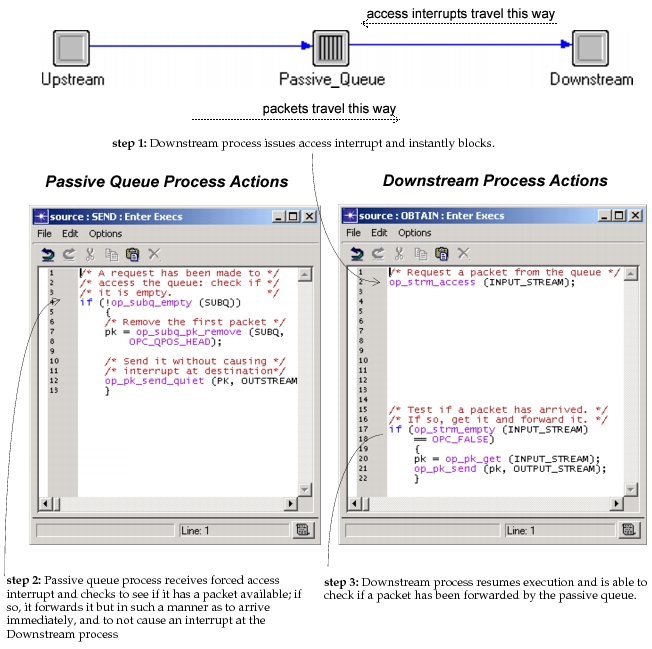
As shown in Figure 87, issuing a forced interrupt causes the process that issues it to be temporarily suspended so that the Simulation Kernel can begin executing the process receiving the interrupt. After the work of the forced process is completed, the suspended process can resume at the statement following the one that originated the action. In other words, from the point of view of the process that generates the forced interrupt, the entire event and all the external actions that it causes are subsumed within one KP call (in this case op_strm_access()).
Key Concept—Two types of events may be submitted for execution. Scheduled events can execute at any future time, including the current time. The Simulation Kernel decides when to execute them based on time and priority. Forced events occur immediately, even if other events are pending for the current time.
Additionally, Figure 87 illustrates another event mechanism implemented by the KP op_pk_send_quiet() and used by the process that responds to the forced interrupt. Because the passive queue process is invoked while the downstream process is suspended, and the downstream process will expect a packet to be present as soon as the call to op_strm_access() has returned, the packet must be forwarded in an immediate way. In other words, it would not be useful to use an event-scheduled mechanism (such as op_pk_send()) to forward the packet because the packet’s delivery would be deferred until sometime after both events had completed, and therefore would not appear in the downstream process’s input stream. In addition, the Simulation Kernel does not support the application of forced interrupts to processes that are already suspended as a result of issuing forced interrupts; this type of interaction may cause problems in terms of continual execution feedback loops as well as multithreaded execution of one process. Therefore, the packet must be forwarded without causing an interrupt for the suspended downstream process. The combined characteristics of immediate execution and lack of interrupt are provided by the class of events referred to as quiet. Currently the Simulation Kernel provides only two KPs that generate quiet events: op_pk_send_quiet() and op_pk_deliver_quiet().
In most cases, the interrupt method is selected by using a particular KP; however, packet streams and statistic wires, which connect modules in the node domain, support the designation of an interrupt method as one of their attributes. For statistic events, the interrupt method is always specified by the “intrpt method” attribute of the statistic wire of interest. For stream events, the selection of an interrupt method by a particular KP overrides any attribute assigned to the packet stream of interest; however, the packet stream’s “intrpt method” attribute may be used to control the interrupt method when the source module is not a queue or processor (i.e., the source module is a receiver).
Note that not all event types support each interrupt method. The following table lists the methods supported by each event type. Note that any event that is specified for a future time (that is, delayed by more than zero seconds from the present time) is necessarily a scheduled event. The forced and quiet methods may only be used for events intended to execute immediately.
Table 42: Support for Interrupt Methods by Event Type
| Event Type | Scheduled | Forced | Quiet |
|---|---|---|---|
| self | ✓ | ||
| stream | ✓ | ✓ | ✓ |
| statistic | ✓ | ✓ | |
| regular | ✓ | ||
| failure | ✓ | ||
| recovery | ✓ | ||
| begin simulation | ✓ | ||
| end simulation | ✓ | ||
| access | ✓ | ||
| remote | ✓ | ✓ | |
| procedure call | ✓ | ||
| multicast | ✓ | ||
| process | ✓ | ||
| esys interface | ✓ |
Key Concept—A third type of event, called Quiet, is similar to the forced event in that it is executed immediately. However, when it is executed, it does not generate an interrupt for the destination object. The forced event merely delivers data to the destination object. The data is processed later when the object receives a scheduled or forced event.
Interrupt Steering
Processor and queue modules are the node domain elements that allow the modeler to implement customized behavior. Each processor or queue can execute multiple processes that respond to interrupts according to their corresponding process models. Initially, each module executes only one process, known as the root process, whose type is specified by the “process model” attribute of the module. However, because processes may create (and destroy) other processes that execute within the same module, the number of actual processes in a module may vary with time.
When it is interrupted, a process may choose to invoke any other process to do part or all of the actions required by the interrupt. Therefore, one possible strategy is to have all interrupts arrive at one process that acts as a dispatcher; based on the attributes of the interrupt, the manager process may invoke the correct process. However, in general it is more convenient, more efficient, and simpler to directly invoke the process that will do the primary actions associated with an interrupt.
By default, all interrupts arriving at a queue or processor module are directed toward the root process, with the exception of self interrupts and process interrupts which are always intended for particular processes; self interrupts always return to the process that scheduled them, and process interrupts incorporate a destination process in their specification. However, the Simulation Kernel provides two mechanisms to steer the interrupts towards processes other than the root process. These two mechanisms must be dynamically activated by a module’s processes because the only interface they provide relies on Kernel Procedures; in other words, when the simulation begins, the default conditions always prevail, meaning that the root process is the implicit recipient of all interrupts. The mechanisms that are provided are called interrupt type registration and interrupt port registration. The term registration refers to the fact that the processes themselves inform the Simulation Kernel how their module’s interrupts should be steered. Both interrupt-steering mechanisms select a process among those in the module based on certain attributes of the interrupt. When the properties overlap, interrupt-port registration is given higher priority.
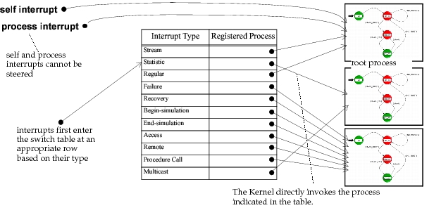
Interrupt type registration considers only the type of interrupt to select a process. A process may register itself or another process as the recipient for interrupts of a particular type arriving at the module of interest. The Kernel Procedure used to do this registration is op_intrpt_type_register(), which is fully documented in “Interrupt Package” on page 1. The type-registration mechanism can be viewed as a bank of switches into which interrupts enter when they first arrive at a module; the switches analyze the type of the interrupt and select a process within the module to receive the first invocation. Initially, all switches point to the root process of the module, but the switches may be reconfigured by correct calls to sub-object This view of the interrupt type registration mechanism is shown in the following figure.
Figure 88: Interrupt Type Registration Mechanism
Interrupt port registration can affect only stream and statistic interrupts. For both of these types, steering is based not only on the type but on the arrival port. The port of an interrupt is simply the input stream on which a packet is arriving in the case of a stream interrupt, and the input statistic attached to the active statistic wire in the case of a statistic interrupt. In both cases, the port is a positive integer index. Interrupt port registration is performed by calling the Kernel Procedure sub-object. See Chapter 11 “Interrupt Package” on page 1 for more information about this procedure.
The application of interrupt port registration is to separate processing of different physical arrivals based on some prior knowledge of their significance. For instance, if its known that packets from a higher level application arrive on input stream number 0 and packets from a physical channel arrive on input stream number 1, a separate process can be created to handle each, rather than creating one process that is capable of handling both source of interrupts on an asynchronous basis. This technique can substantially simplify process model design.
Key Concept—Because multiple processes can exist within one module, the Simulation Kernel must decide to which process each event for that module should be delivered. By default the root process receives all events. However, specific processes can request to receive particular events directly based on the event type and in some cases, the event port (i.e., the input stream or statistic).
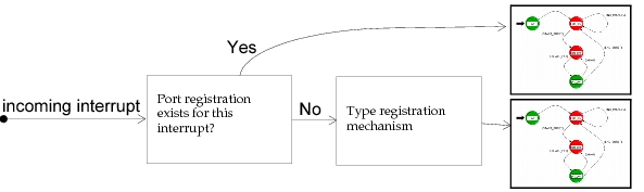
Because port registration applies to stream and statistic interrupts, and type registration can apply to these interrupts as well, the Simulation Kernel must accord priority to one mechanism over the other. The port registration mechanism is more specific because different interrupts of the same type may be affected differently; therefore by allowing port registration to override type registration the Kernel can support combinations of the two mechanisms. In other words, stream and statistic interrupts in general may be steered toward a particular process due to the type-registration mechanism, while particular interrupts of these types may be steered differently. The following figure shows the Kernel selection mechanism when both type and port registration are employed.
Figure 89: Steering Based on Port Registration Is Given Precedence
The effects of interrupt type registration are easily undone by re-registering the root process of a module, because initially the root process is registered for all interrupt types. However, a special KP, op_intrpt_port_deregister() is required to reestablish prior conditions after op_intrpt_type_register() has been used, because simply installing the root process for a particular interrupt type and port may override a simultaneous type registration. See the descriptions of these KPs in Chapter 11 “Interrupt Package” on page 1 for more information about reversing the effects of the interrupt steering mechanisms.
Interrupt steering is a powerful technique for implementing complex processes that deal with a large number of interrupts of different types and that arrive on different ports. The effective use of the two mechanisms described in this section can allow the modeler to decompose a process’s functionality and implement instead as a group of smaller processes, each of which is more easily represented. See Chapter 5 “Process Domain” on page 165 for more information about the application of interrupt steering.
Event Prioritization for Simultaneous Event Execution
As mentioned earlier in this section, the Simulation Kernel’s event management policies support the execution of multiple events at the same simulation time. Simultaneous event scheduling can occur as a result of several phenomena:
- A model might contain synchronously operating components – Different components in the same node or in different nodes can do activities concurrently due to regular timing imposed throughout the system. This is commonly the case in digital hardware systems where many components are driven by the same clock. Many communication systems operate in a similar fashion, using pre-designated slot times to transmit and receive messages.
- Unrelated events might coincide on an irregular basis – Events occurring in different nodes, or even at the same module, can be scheduled at the same time, even if these events are issued by different sources that are independent of one another. This is commonly the case when only a small number of timing increments are used in a simulation (i.e., fixed transmission times, propagation delays, interarrival times, timer intervals, etc.), because it is likely that different combinations of these increments will add up to yield the same simulation time for a new event.
- Actions taken during an event can generate new events at the same simulation time – This occurs frequently due to idealization of communication or invocation mechanisms which are modeled as requiring no time to complete. For example, a packet sent over a packet stream with delay equal to zero will result in a new event at the receiving module at the exact same time as the event during which the packet was sent. Note that due to simultaneous events of this type, the number of events at a given time cannot be known until the last event at that time has completed execution (i.e., new events at the same time can be introduced).
Discrete event simulations typically are designed to execute on a serial computer and therefore can implement only one event at a time. Thus, the concurrency of simultaneous events must be emulated by maintaining the simulation time at a constant value until all events at a given time have executed. In certain cases, the behavior of a model might be significantly affected by the order in which the simultaneous events are executed.
For example, consider once again a process that sends packets and expects acknowledgments in return; a timer is set using a self interrupt to indicate that a retransmission is necessary after a certain period. Now consider the case where the acknowledgment and the timer expire at the same simulation time. If the self interrupt representing the timer’s expiration is received by the process first, a retransmission may be issued; on the other hand, if the stream interrupt associated with the acknowledgment packet is received first, the acknowledgment will be judged to have arrived within the required time limit, and the retransmission will not be issued. While this type of behavioral ambiguity may be tolerable for certain simulations, for other models only one of the possible behaviors may be correct. In addition, the unpredictability of the model’s operation can hinder simulation tracing efforts during model validation or debugging.
To provide for deterministic control of the order in which events are executed, the Simulation Kernel provides two ordering mechanisms: object prioritization and interrupt prioritization. In addition, the “event_order_method” preference allows a choice between strict and partial ordering.
Note: Object prioritization is used only with sequential simulations. The parallel simulation kernel does not use the priority and super priority attributes.
Object Prioritization
Object prioritization is useful to provide a deterministic ordering for events that occur at the same time, but at different modules. The Simulation Kernel determines precedence based on a priority rating assigned to each module. The priority rating of a module is a function of two factors:
- The module’s “priority” attribute (queues and processors only).
- The priority of the node and immediate subnetwork objects that encompass the module (the priorities of higher-level subnetworks, beyond the one that immediately encompasses a module, are not considered).
Priority is evaluated on a hierarchical basis, with greater importance attributed to the higher level object attributes. Therefore, a module can have a higher “priority” attribute than another, and yet have a lower aggregate priority rating if the second module is encompassed within a subnet with a higher “priority” attribute than the first module’s subnet.
Only one exception is made to this hierarchical priority scheme: a boolean attribute called “super priority” is provided on queue and processor modules. A module with an “enabled” value for “super priority” always has a higher overall priority rating than one whose value is “disabled”. The general rule for comparing event priority is listed in the following table. The notation is as follows: Subnet (X) is the most immediate subnet of X (that is, the immediate parent of X’s node); Node (X) is the node in which A is included; X. “priority” is the value of the “priority” attribute of X.
Table 43: Criteria for Module A Having Higher Priority Rating Than Module B
- A.super priority = enabled and B.super priority = disabled
- Subnet (A).priority > Subnet (B).priority
- Subnet (A).priority = Subnet (B).priority and
Node (A).priority > Node (B).priority - Subnet (A).priority = Subnet (B).priority and
Node (A).priority = Node (B).priority and
A.priority > B.priority
If any two events are simultaneously present in the event list and scheduled for exactly the same simulation time, and if the events are scheduled for two different modules, the event scheduled for the module with higher aggregate priority rating is executed first. Note that it is an important condition that both events be present together in the event list because it is usually impossible to anticipate the arrival of simultaneous events of type 3 above. For instance, it is possible for a low priority module to execute, then schedule an event for a higher priority module with no delay. The execution sequence interrupts the lower priority module first, and this may seem paradoxical to a user tracing through the events of the simulation; however this is normal behavior because the higher priority module’s event was not known to the Simulation Kernel until after the lower priority event had already begun execution.
Interrupt Prioritization
Interrupt priorities are used to establish an order for events that occur at the same time as well as at the same process (not the same module). Classification of interrupts is based on an integer priority value assigned to a combination of interrupt type and interrupt code. Each process can adjust its own priorities (but not those of other processes) by calling the KPs op_intrpt_priority_set() and op_intrpt_priority_set_next(). Each of these KPs allows the specification of an interrupt type and an interrupt code as well as an integer priority value. Higher numerical priority values correspond to higher precedence of execution for the specified interrupt type and code; negative and positive priority values are allowed. The default priority value for all interrupt type and code combinations is zero.
Natural Order
For both object and interrupt priority mechanisms, if two events have the same simulation time and the same priority rating, precedence is given to the event that was inserted into the event list first. This ordering of event execution is termed natural order. Natural ordering is also the default ordering policy which is applied when neither priority mechanism is used.
Key Concept—When two events are scheduled for identical simulation times, the Simulation Kernel must decide which one to execute first. Several priority mechanisms can be used to establish precedence when needed. Object priority separates events occurring at different objects. Interrupt priority separates events occurring at the same object. When priorities are equal or unused, the natural order of scheduling is followed.