Data Collection and Simulation
The objective of most modeling efforts is to obtain measures of a system’s performance or to make observations concerning a system’s behavior. Modeler supports these activities by creating an executable model of the system. Provided that the model is sufficiently representative of the actual system, Modeler allows realistic estimates of performance and behavior to be obtained by executing simulations. Several mechanisms are provided to collect the desired data from one or more simulations of a system.
For more information, see
Simulation Output Data Types
Discrete event simulations are capable of producing many types of output. Of course, because of the general programmability of process models and link models, developers can define their own types of output files, including text reports, proprietary binary files, etc. However, in most cases, modelers use the types of data directly supported by discrete event simulations:
Key Concept—Modelers can take advantage of the programmability of Riverbed models to create proprietary forms of simulation output, if desired. However, in most cases, users work with the output that can be provided automatically by discrete event simulations. These are: output vectors, output scalars, and animations.
Output Vectors
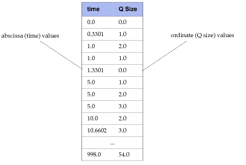
The types of data that can be collected have several different forms. The most common result extracted from a simulation is called an output vector, which is simply a collection of pairs of real values, called entries. An output vector, often called simply a vector, contains an arbitrarily-sized list of entries collected during one simulation run. The first value in the entries can be thought of as the independent variable and the second as the dependent variable. These are referred to as the abscissa and the ordinate, respectively. In the majority of cases, the independent variable of a vector is simulation time, which increases monotonically as a simulation’s execution progresses. In other words, most vectors represent the value of some quantity of interest as it varies over time. Under certain conditions, it is interesting to create vectors that have abscissa variables other than time; this topic is described later in this manual. The following figure depicts a typical data set contained in a vector. Note that it is possible for a vector to store multiple ordinate values with the same abscissa value.
Key Concept—Output vectors represent time-series simulation data. They consist of a list of entries, each of which is a time-value pair.
Figure 11: Output Vector Contents
Output Scalars
In contrast to vectors, scalar statistics are individual values. Typically, scalar statistics are averages, probabilities, or peak values derived from a collection of measurements. Examples include the average or peak size of a queue, the mean end-to-end delay of packets, the proportion of calls blocked or dropped, the mean call duration, etc. Based on these examples it is clear that many scalars are simply properties or statistics of the set of value pairs obtained in an output vector. In other words, given all of the values in an output vector, a number of interesting scalars can be computed and recorded by a simulation. Note that it is not usually necessary to record all the values in a vector to compute a scalar that reflects the entire data set. For example, the mean ordinate value of a vector can be obtained by maintaining a running sum of the vector’s values as they become available and dividing by a running count of the number of values recorded. Therefore, recording scalars is often much more efficient in terms of disk space and disk I/O than recording vectors.
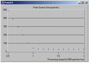
Scalars are typically only of limited use when taken as individual data points. Instead, the usual practice is to combine scalars recorded over multiple simulations to form a graph or curve that indicates how a system variable varies as a function of other system parameters. Both the dependent and the independent system variables, used to generate such a graph, are recorded as scalars. For example, a typical graph generated in performance analysis is Throughput vs. Offered Load, which indicates how well a network is able to deliver the data that it is requested to deliver, as the amount of data increases. Here the Offered Load scalar is an independent variable that is varied as an input to each simulation. Throughput is measured over the course of the simulation and its final value (because it is already an average) is recorded as another scalar.
Key Concept—Scalar statistics are individual values that represent a metric of interest. They are often derived from vector statistics, as an average, peak value, final value, or other statistic. Typically, one value for each scalar statistic is recorded during a simulation; when many simulations are run, their scalar outputs are combined to form a graph.
When Throughput is graphed against Offered Load, each point in the graph is formed by taking an abscissa and an ordinate value from the respective scalar statistics within the same simulation run. Each point of the graph usually corresponds to a new simulation run. The following figure shows a typical plot generated from scalar values.
Figure 12: Plot of Scalar Statistic Values
Application-Specific Statistics
Both scalar and vector statistics can be computed and recorded automatically for a set of predefined statistics. Predefined statistics are related to values that can be measured at specific objects within the model. This includes statistics such as queue sizes, link throughputs, error rates, and queuing delays. In addition, it is common for models to compute application-specific statistics during a simulation and record them in vector output files. These statistics can be computed in a completely general manner, taking into account events that have occurred, the current state of the system, the content of packets, etc.
Custom statistics may be declared by process models, in which case Modeler adds them to the set of built-in statistics of queues and processors that make use of those process models. The custom statistics can have a scope which is local or global. A locally-scoped statistic is maintained separately for each processor or queue that declares it. This is appropriate for recording information that relates only to events at a particular location, such as the utilization of a CPU on a particular server. In contrast, a global statistic is shared and contributed to by many entities in the model, it is appropriate for recording information that relates to the performance or behavior of the system as a whole. A typical example of a global statistic is the end-to-end delay of all application data transported by a network, regardless of origin or destination.
Key Concept—Modeler supports predefined statistics that are typically of interest in simulation studies. However, many projects require customized statistics, computed in a manner specific to the application. Modeler supports both local (related to an object) and global (related to overall system) application-specific statistics.
Animations
In addition to numerical forms of output, discrete event simulations can provide a visual analysis of a network model’s behavior. An animation is a dynamic graphical representation of selected events that occurred during a simulation. The events may be depicted within a diagram from the Network, Node, or Process domain, or simply in an empty window.
A discrete event simulation can be configured to generate certain types of predefined animations automatically. The Animation Kernel Procedure package also provides the ability to program sophisticated animations that represent simulation events in a customized manner. The kernel procedures of the Animation package include general drawing as well as Modeler-specific graphics to provide a flexible animation capability.
Both automatic and custom animations can be viewed interactively during a simulation run or afterwards in a “playback” mode. See the documentation for the Animation package Kernel Procedures in Discrete Event Simulation API Reference Manual and the animation program description in Animation Viewers Reference Manual for more information about developing and viewing animations.
Key Concept—Discrete event simulations can generate animations that you can view during the run or afterwards. Several forms of predefined or automatic animations are provided (packet flows, node movement, state transitions, and statistics). You can also program your own detailed, customized animations.
Selecting Data for Collection
Because standard models typically contain a very large number of potential statistics and animations of interest, collection mechanisms are not active by default when a simulation is executed. Instead, Modeler provides a mechanism to explicitly activate particular statistics or animations so that they will be recorded in appropriate output files. This is accomplished by specifying a list of probes when running a simulation. Each probe indicates that a particular scalar statistic, vector statistic, or form of animation should be collected. Probe lists are defined using the Choose Results operation in the Project Editor. You can also define advanced forms of probes in the Probe Editor, which is described later in this manual.
In addition to enabling a statistic or animation, a probe can specify options that affect how data is collected. For statistics, commonly used options include restricted time-windows for data collection, on-the-fly data-reduction, and modified statistic names. For animations, probes allow you to define window geometry and several type-specific animation options. For more information about probes, see Chapter 10 “Simulation Design” on page 375.
Key Concept—Simulations can potentially generate vast amounts of output data. Therefore, by default, each source of output data is disabled. Modelers must explicitly enable particular output data for collection. Results for collection are defined by probes, which also specify options that affect the manner in which results are collected or displayed.