Model Specification
Model specification is the task of developing a representation of the system that is to be studied. Modeler supports the concept of model reuse so that most models are based on lower level models developed beforehand and stored in model libraries. Ultimately, however all models are based on the basic concepts and primitive building blocks supplied by the Modeler environment.
For more information, see:
Specification Editors
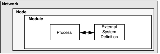
Modeler supports model specification with a number of tools, called editors, which capture the characteristics of a modeled system’s behavior. Because it is based on a suite of editors that address different aspects of a model, Modeler is able to offer specific capabilities to address the diverse issues encountered in networks and distributed systems. To present the model developer with an intuitive interface, these editors handle the required modeling information in a manner that is parallel to the structure of real network systems. Therefore, the model-specification editors are organized hierarchically. Models built in the Project Editor rely on elements specified in the Node Editor; in turn, when working in the Node Editor, you use models defined in the Process Editor and External System Editor. The remaining editors are used to define various data models, typically tables of values, that are later referenced by process- or node-level models. This organization is reflected in the following list.
- Project Editor – Develop network models. Network models are made up of subnets and node models. This editor also includes basic simulation and analysis capabilities.
- Node Editor – Develop node models. Node models are objects in a network model. Node models are made up of modules with process models. Modules may also include parameter models.
- Process Editor – Develop process models. Process models control module behavior and may reference parameter models.
- External System Editor – Develop external system definitions. External system definitions are necessary for cosimulation.
- Link Model Editor – Create, edit, and view link models.
- Packet Format Editor – Develop packet formats models. Packet formats dictate the structure and order of information stored in a packet.
- ICI Editor – Create, edit, and view interface control information (ICI) formats. ICIs are used to communicate control information between processes.
- PDF Editor – Create, edit, and view probability density functions (PDFs). PDFs can be used to control certain events, such as the frequency of packet generation in a source module.
Key Concept—Riverbed models are structured hierarchically, in a manner that parallels real network systems. Specialized editors address issues at different levels of the hierarchy. This provides an intuitive modeling environment and also permits re-use of lower level models.
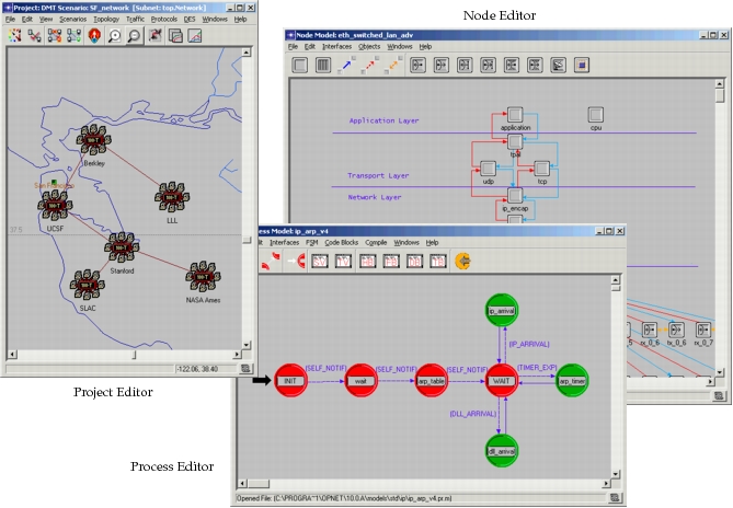
Modeler makes use of graphical specification of models wherever appropriate. Therefore, the model-specification editors all present a graphical interface in which the user manipulates objects representing the model components and structure. Each editor has its own specific set of objects and operations that are correct for the modeling task on which it is focused. For instance, the Project Editor uses node and link objects; the Node Editor provides processors, queues, transmitters, and receivers; and the Process Editor is based on states and transitions. As a result, the diagrams developed in each editor have a distinct appearance, as shown in the following screen samples.
Figure 2: Graphical Editors for Network, Node, and Process Models
Modeling Domains
The Network, Node, Process, and External System modeling environments are sometimes referred to as the modeling domains of Modeler because they span all the hierarchical levels of a model. The remaining specification editors correspond to no particular modeling domain because they mainly support the three principal editors. As mentioned earlier, the capabilities offered by the modeling domains mirror the types of structures found in an actual network system; the issues addressed by each domain are summarized in the following table and then briefly described in the remainder of this section.
Table 1: Modeling Domains
| Domain | Editor | Modeling Focus |
|---|---|---|
| Network Domain | Project | Network topology described in terms of subnetworks, nodes, links, and geographical context. |
| Node Domain | Node | Node internal architecture described in terms of functional elements and data flow between them. |
| Process Domain | Process | Behavior of processes (protocols, algorithms, applications), specified using finite state machines and extended high-level language. |
| External System Domain | External System | Interfaces to models provided by other simulators running concurrently with a discrete event simulation (a cosimulation). |
Network Domain
The Network Domain’s role is to define the topology of a communication network. The communicating entities are called nodes and the specific capabilities of each node are defined by designating their model. Node models are developed using the Node Editor, described later in this section. Within one network model, there may be many nodes that are based on the same node model; the term node instance is used to refer to an individual node to distinguish it from the class of nodes sharing the same model. However, in general, when the term node is used by itself, in the context of the network domain, it can be assumed that a node instance is being referred to, rather than a node model.
A network model may make use of any number of node models. Modeler does not place restrictions on the types of nodes that can be deployed in a communication network; instead it adopts an open approach whereby modelers can develop their own library of node models to use as building blocks for network models. There are no limits on the number of node models or node instances that a network model can contain (other than those imposed by workstation memory limitations).
Key Concept—A network model may contain any number of communicating entities called nodes. Nodes are instances of node models, developed using the Node Editor. Modelers can develop their own library of customized node models, implementing any functionality they require.
The Project Editor can provide a geographic context for network model development. You can choose locations on world or country maps for the elements of wide-area networks and can use dimensioned areas for local-area networks. In addition to providing an intuitive environment for deploying the components of a network model, this feature provides an intrinsic notion of distance, which allows automatic calculation of communication delays between nodes.
The basic object used to build network models is the fixed communication node. In Modeler, this is the only type of node available. Fixed nodes can be assigned arbitrary locations, but during a simulation their location may not change. The optional Wireless functionality adds capability for mobile and satellite nodes, as described in Chapter 2 “Modeling Wireless Networks” on page 3. Mobile nodes can be assigned predefined trajectories that specify their positions as a function of time throughout a simulation run; similarly, satellite nodes are assigned orbits that prescribe their motion. With the Wireless functionality, simulations can involve all three types of nodes.
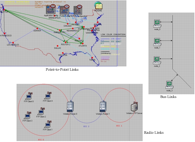
Most nodes require the ability to communicate with other nodes to do their function in a network model. Several different types of communication link architectures are provided to interconnect nodes that communicate with each other. Modeler provides simplex (unidirectional) and duplex (bidirectional) point-to-point links to connect nodes in pairs and a bus link to allow broadcast communication for arbitrarily large sets of fixed nodes. The Wireless functionality adds the capability for fixed, satellite, and mobile nodes to communicate with each other via radio links. While bus and point-to-point links are modeled as explicit objects that you must create, radio links are dynamically evaluated based on characteristics of the communicating nodes. As will be described in later sections, each type of link can be customized by editing parameters or supplying new logic for the underlying link models. The following figure shows some typical network model diagrams involving each of the supported link types.
Key Concept—Network models consist of nodes and links that can be deployed within a geographical context. Modeler comes with fixed nodes and point-to-point and bus links; the Wireless functionality adds mobile and satellite nodes and radio links.
Figure 3: Network Models with Point-to-Point, Bus, and Radio Links
To break down complexity and to simplify network protocols and addressing, many large networks make use of an abstraction known as a subnetwork. A subnetwork is a subset of a larger network’s devices that forms a network in its own right. Modeler provides fixed, mobile, and satellite subnetworks to enhance network models. These subnetworks can then be connected by different types of communication links, depending on the type of subnetwork. The larger network can then be viewed as a network of its subnetworks. This abstraction can be carried out at many levels. In other words, one can form networks of subnetworks, which in turn are formed of other subnetworks, and so on. At the bottom of this hierarchy, the lowest level subnetwork is composed only of nodes and links, but no other subnetworks.
Key Concept—Fixed, mobile, and satellite subnetwork objects provide hierarchy in the network model and are used to break down complexity into multiple levels. Subnets can contain various combinations of nodes, links, and other subnets, and can be nested to any depth.
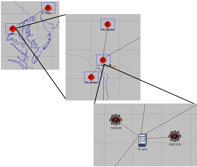
In network models, subnetworks can be nested to an unlimited depth to construct complex topologies. The following set of diagrams, captured in the Project Editor, illustrate the use of fixed subnetworks to model hierarchical networks.
Figure 4: A Hierarchical Network with Two Levels of Subnetworking
Node Domain
The Node Domain provides for the modeling of communication devices that can be deployed and interconnected at the network level. In Modeler terms, these devices are called nodes, and in the real world they may correspond to various types of computing and communicating equipment such as routers, bridges, workstations, terminals, mainframe computers, file servers, fast packet switches, satellites, and so on.
Node models are developed in the Node Editor and are expressed in terms of smaller building blocks called modules. Some modules offer capability that is substantially predefined and can only be configured through a set of built-in parameters. These include various transmitters and receivers allowing a node to be attached to communication links in the network domain. Other modules, called processors, queues, and external systems, are highly programmable, their behavior being prescribed by an assigned process model. Process models are developed using the Process Editor.
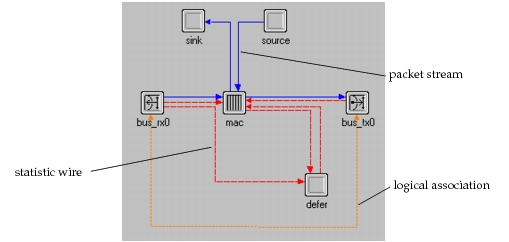
A node model can consist of any number of modules of different types. Three types of connections are provided to support interaction between modules. These are called packet streams, statistic wires (also sometimes referred to as streams and statwires, respectively), and logical associations. Packet streams allow formatted messages called packets to be conveyed from one module to another. Statistic wires convey simple numeric signals or control information between modules, and are typically used when one module needs to monitor the performance or state of another. As will be described later in this manual, both packet streams and statistic wires have parameters that may be set to configure aspects of their behavior. Logical associations identify a binding between modules. Currently, they are allowed only between transmitters and receivers to indicate that they should be used as a pair when attaching the node to a link in the Network Domain. The following figure shows a typical node model that includes the three types of connections.
Key Concept—Node models consist of modules and connections. Modules are information sources, sinks, and processors. Some modules have pre-defined behavior; processor and queue modules are programmable via their process model. Connections (packet streams and statistic wires) allow information to flow between modules.
Figure 5: Node Model Employing Packet Streams, Statistic Wires, and Logical Associations
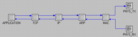
The modeling paradigm selected for the Node Domain was designed to support general modeling of high-level communication devices. It is particularly well suited to modeling arrangements of stacked or layered communication protocols. In the Node Editor, a device that relies on a particular stack of protocols can be modeled by creating a processor object for each layer of that stack and defining packet streams between neighboring layers, as shown in the following diagram for the familiar TCP/IP stack.
Figure 6: Possible Representation of TCP/IP Protocol Stack
Process Domain
As indicated in the description of the Node Domain, queue and processor modules are user-programmable elements that are key elements of communication nodes. The tasks that these modules execute are called processes. Because it has a set of instructions and maintains state memory, a process is similar to an executing software program. Processes in Modeler are based on process models that are defined in the Process Editor. The relationship between process model and process is similar to the relationship between a program and a particular session of that program running as a task (in fact, the term process is used in many operating systems as well). Just as nodes created in the Project Editor are instances of node models defined with the Node Editor, each process that executes in a queue, processor, or esys module is an instance of a particular process model.
Key Concept—Process models define behavior for programmable modules. A process is an instance of a process model and operates within one module.
The process modeling paradigm of Modeler supports the concepts of process groups. A process group consists of multiple processes that execute within the same processor or queue. When a simulation begins, each module has only one process, termed the root process. This process can later create new processes which can in turn create others as well, etc. When a process creates another one, it is termed the new process’ parent; the new process is called the child of the process that created it. Processes that are created during the simulation are referred to as dynamic processes.
Modeler places no limits on the number of processes that may be created in a particular processor or queue. Processes may be created and destroyed based on dynamic conditions that are analyzed by the logic of the executing processes. This paradigm provides a very natural framework for modeling many common systems. In particular, multitasking operating systems where the root process represents the operating system itself and the dynamically created processes correspond to new tasks; and multi-context protocols where the root process represents a session manager, for example, and each new session that is requested is modeled by creating a new process of the correct type.
Key Concept—Initially, each programmable module contains only one process; however, processes can create additional child processes dynamically. These can in turn create additional processes themselves. This paradigm is well-suited to modeling systems with dynamically instantiated contexts, like certain protocols, or multi-tasking operating systems.
Only one process can be executing at any time. A process is considered to be executing when it is progressing through new instructions that are part of its process model. When a process begins execution it is said to be invoked. A process that is currently executing can invoke another process in its process group to cause it to begin executing. When this happens, the invoking process is temporarily suspended until the invoked process blocks. A process blocks by indicating that it has completed its processing for its current invocation. After the invoked process has blocked, the invoking process resumes execution where it had left off, in a manner similar to the procedure-call mechanism in a programming language such as C.
Processes in Modeler are designed to respond to interrupts and/or invocations. Interrupts, which are described in detail in later sections of this manual, are events that are directed at a process and that may require it to take some action. They may be generated by sources external to a process group, by other members of a process group, or by a process for itself. Interrupts typically correspond to events such as messages arriving, timers expiring, resources being released, or state changes in other modules. After a process has been invoked due to an interrupt, it may invoke other processes in the group and these may in turn invoke other processes, etc. An interrupt’s processing is completed when the first process that was invoked blocks.
Key Concept—Processes respond to interrupts, which indicate that events of interest have occurred such as the arrival of a message or the expiration of a timer. When a process is interrupted, it takes actions in response and then blocks, awaiting a new interrupt. It may also invoke another process; its execution is suspended until the invoked process blocks.
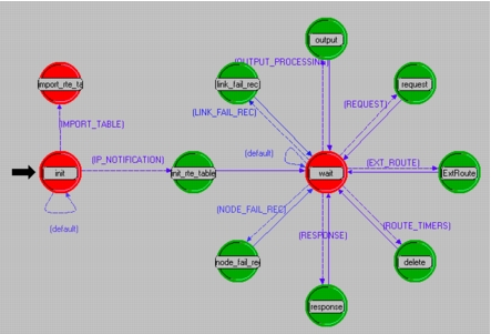
The Process Editor expresses process models in a language called Proto-C, which is specifically designed to support development of protocols and algorithms. Proto-C is based on a combination of state transition diagrams (STDs), a library of high-level commands known as Kernel Procedures, and the general facilities of the C or C++ programming language. A process model’s STD defines a set of primary modes or states that the process can enter and, for each state, the conditions that would cause the process to move to another state. The condition needed for a particular change in state to occur and the associated destination state are called a transition. The following example, taken from the Process Editor, shows the relationship between states and transitions in a process model’s STD.
Figure 7: State Transition Diagram in the Process Editor
Proto-C models allow actions to be specified at various points in the finite state machine. The actions can be general in nature because they are expressed as C or C++ statements. Because Proto-C is focused on modeling protocols and algorithms, it also provides an extensive library of over 300 Kernel Procedures (also known as KPs) that can be invoked to do commonly needed actions. Kernel Procedures are grouped into packages of related functions. The following table shows some of the capabilities provided by the Kernel Procedure libraries.
Key Concept—Process models are expressed in Proto-C, a language combining graphical state-transition-diagrams, embedded C/C++ language data items and statements, and a library of Kernel Procedures that provide commonly needed functionality for modeling communications and information processing systems.
Table 2: Major Simulation Kernel Procedure Packages
| Package | Applications |
|---|---|
| Anim | Support for custom animation development |
| Dist | Probability distribution and random number generation |
| Esys | Read from and write to external system interfaces |
| Ev | Event list and event property query; event cancellation |
| Ici | Formal interfaces between processes; association of information with interrupts |
| Id | Identification of objects |
| Ima | In-simulation query and modification of object attributes |
| Intrpt | Query of interrupt properties; control of interrupt handling |
| Pk | Creation, destruction, modification, analysis, and transmission of packets |
| Prg | Programming support: linked lists, memory, string manipulation, debugging |
| Pro | Creation, invocation of processes; process group shared memory |
| Q | Queueing statistics; high-level queueing operations |
| Rte | Basic routing support for static routing implementations |
| Sar | Segmentation and reassembly of packets |
| Sim | Simulation control: customized messaging, simulation execution control |
| Stat | Custom statistic generation; intermodule signalling via statistic wires |
| Strm | Communication between modules via packet streams, packet delivery |
| Subq | Low-level queueing operations: enqueueing, dequeueing, statistics, etc. |
| Tbl | Accessing of tabular data: antenna patterns, modulations |
| Td | Setting and getting of transmission data for custom link models |
| Topo | Query of model topology (for example, automatic discovery and configuration) |
| Vvec | Create and manipulate value vectors |
The state transition diagram representation of Proto-C is well suited to the specification of an interrupt-driven system because it methodically decomposes the states of the system and the processing that should take place at each interrupt. STDs developed in the Process Editor have a number of extensions beyond the capabilities offered by traditional state-transition diagram approaches:
- State Variables – Processes maintain private state variables with named variables of arbitrary data types, including Modeler-specific, general C/C++ language, and user-defined types. This capability allows a process to flexibly maintain counters, routing tables, statistics related to its performance, or messages requiring retransmission. Arbitrary combinations of state variable values may be used in all decisions and actions implemented by a process.
- State Executives – Each state of a process can specify arbitrarily complex actions associated with the process entering or leaving that state. These actions, called state executives, are expressed with the full flexibility of the C/C++ language. Typical actions include modifying state information, creating or receiving messages, updating the contents of and sending messages, updating statistics, and setting or responding to timers.
- Transition Conditions – Transition condition statements, which determine whether a transition should be traversed, may be expressed as general C/C++ language booleans that make reference to properties of a new interrupt as well as to combinations of state variables.
- Transition Executives – Transitions may specify general actions, called executives, which are implemented each time that they are traversed.
A process model can define parameters, called attributes, that are used after it is instantiated as a process to customize aspects of its behavior. This technique fosters reuse of process models for various purposes by avoiding hardwired specification where possible. For instance, a process model that performs window-based flow control, may be defined with the window size as an attribute, so that it is reusable in different situations requiring different values of the window size.
External System Domain
The esys module mentioned in the description of the Node Domain encompasses the mechanism for communicating with other simulators and allowing them to interact with a discrete event simulation. This interaction, called a cosimulation, means that the two simulators can exchange data while running synchronously. Part of the role typically played by a module inside a node is instead played by a simulator external to Modeler. For esys modules, the process model controls Modeler’s interaction with the external system. Esys modules have all the capabilities of both processors and queues.
Figure 8: Relationship of Hierarchical Levels in Models
To the simulation, an external system is a black box. While Modeler can feed data to the external system and receive data from it, the other simulator has complete control of the data after it arrives.
An esys module consists of two primary parts:
- External system – The external system definition specifies (via a simulation description file) how the cosimulation should be built and defines the esys interfaces that will exchange data with the external code. They can accept data from external code, send data to external code, or do both. An esys interface normally contains one value at any given time, and both Modeler and the external code have access to that value. An esys interface can contain only one value at a time, unless it is specifically given more elements, in which case it is called a vector interface. A vector interface can hold as many values as it has elements. The elements within a vector interface are distinguished by index numbers, much as individual positions in an array are referenced by index number.
- Process model – The process model of the esys module places values onto esys interfaces and reads values placed onto the esys interfaces by the external simulator. It serves as the interface between the external code and the rest of the model.
Key Concept—When Modeler runs a cosimulation, its interface with the external code is an external system definition (ESD), represented in the node model by an esys module. ESDs use esys interfaces to send and receive data when communicating with external code.
Models, Objects, and Attributes
The preceding sections describe major model types and objects; this section presents the Modeler object model in more detail. Wherever possible, information is presented independently of modeling domains, except when focusing on examples.
Objects
Objects represent entities that are part of the system of interest. In general, an object is a component, or building block of a model and the object is said to be part of that model. So for example, a processor module is an object that is part of a node model. An object generally plays one or more of the following roles in a model:
Typical roles of an object in a model:
- Specify behavior
- Create information
- Store and manage information
- Process, modify, or relay information
- Respond to events
- Contain other objects
Objects are created by various mechanisms in models. Many result from explicit specification by the user via graphical or programmatic methods. So for example, a link object may be created in a network model by physically dragging it from the Project Editor’s object palette. Other objects are created automatically by the system. For example, subqueue objects are automatically created for a queue object. Similarly, when a node object is created, the objects within the node are also implicitly assumed to exist. Finally, during simulation, some objects are created dynamically by the system or by the model. A process, for example, can be considered an object and may be created at any time by another process to do a task. Dynamic objects are different in many ways than the statically created objects; in particular they offer more specialized interfaces, allowing them to be manipulated in a more efficient manner. Most of the material in this section does not apply to dynamic objects.
Key Concept—Objects are the building blocks of models and appear in each of the modeling domains. Some objects are created explicitly by the user; others are implicitly created by Modeler. During a simulation, certain types of objects can be created dynamically.
Attributes
To achieve predictable and tractable behavior when building a complex many-object system, each object must have a well-defined interface. The interface of an object consists primarily of the attributes that it makes available and the procedures that it supports to access its attributes or to cause it to do actions. Some procedures supported by objects are provided automatically by Modeler; others are programmed by users for specialized needs. Most procedures vary according to object type, so few general comments can be made about them except to say that it is crucial that they have a well-known interface and that they shield users from underlying details of object implementation.
Table 3: Attribute Components
- Name
- Value
- Properties
Attributes are data items used to configure an object and represent the control that the object’s designer has made available to the user. Each attribute has a name that allows it to be referenced uniquely within an object. Each attribute also provides a storage area for the information that is “assigned to it”. This information is called the attribute’s value. Finally, an attribute has a set of properties that specify the rules related to its use, as well as several additional functions. Major attribute properties are enumerated in the following table.
Table 4: Attribute Properties
| Property | Description |
|---|---|
| Data Type | Class of data storage. Modeler supports a variety of numerical and text storage types, as well as a compound attribute whose value is another object. |
| Default Value | Provides a value that can be used in the absence of explicit assignment. |
| Range | For numerical attributes, limits the set of acceptable values to specified bounds. |
| Symbol Map | Lists values and names that represent them. Supports pre-configuration and more meaningful presentation of value choices. Also can be used to limit value choices to a restricted set. |
| Comments | Documents any information desired about the attribute. Generally describes the attribute’s purpose and interface (how it behaves) |
As described in the table, Modeler supports an attribute data type called compound. Compound attributes support nested complex data storage within an object in a very simple way: the value is itself another object. This object can have any number of attributes of its own, including additional compound attributes. Certain built-in objects have compound attributes. For example, queues incorporate subqueues using this mechanism; similarly, transmitters and receivers represent the channels they contain as compound attributes. User-defined models may also create compound attributes for application-specific purposes. A typical use of a compound attribute in a protocol model is to represent a routing or circuit table.
Key Concept—Objects provide attributes as a means of controlling their behavior. The attributes constitute part of the object’s interface. Each attribute has a name, a value, and properties. Properties specify the rules governing the attribute’s use, including its data type, allowable values, suggested values, and documentation.
Models
Many models (network, node, and process) consist largely of objects. At the same time, most objects have a model that confers upon them some or all of their characteristics. The object is an instance of the model because there is a many-to-one relationship between a model and the objects that refer to it. The model defines an object class to which all related objects belong.
Some objects are fundamental and have an implicit model that cannot be changed by the user. For example, state objects in process models are simple objects whose only means of external control is provided by their attributes. Their characteristics and behavior are defined and documented and these constitute their model; however, their fundamental behavior and structure are always similar and cannot be changed. Therefore they have no “model” attribute.
However, several key objects offer a “model” attribute that allows their fundamental behavior and structure to be controlled externally. In fact, altering an object’s model can even cause it to acquire a completely new interface. Indeed, these objects are fundamentally quite generic, and most of their characteristics are obtained from the model to which they refer. The following table lists the objects that support a “model” attribute.
Table 5: Objects Supporting Model Assignment
| Object | Modeling Domain | Model Type |
|---|---|---|
| Node (all types) | Network | Node |
| Link (all types) | Network | Link |
| Processor | Node | Process |
| Queue | Node | Process |
| External System | Node | Process, ESD |
In each of the model types listed in Table 5, a model interface is specified. One of the characteristics transferred to an object from its model is its set of attributes. The model dictates which new attributes will be acquired by the object, and what their names and values will be. Similarly, it can specify values for attributes that intrinsically belong to the object and can also cause these to become hidden from the user. Therefore, the model can completely control the attribute interfaces of the object.
Key Concept—Each object has a behavior and structure that is specified by a model. Models also specify part or all of an object’s interfaces. Some objects have implicit models that cannot be changed; others can be assigned models via their “model” attribute, allowing extensive customization.
Model Attributes and Attribute Promotion
With both models and attributes introduced as concepts, the notion of a model attribute can be defined. In addition to describing objects, attributes can be associated with models to represent a parameter of the model. This was mentioned previously with regard to process models. The importance of providing a parameter for a model lies in increasing the generality of the model. By varying the values of the model’s parameter, a user can alter model behavior without modifying the model. This approach is in contrast to hardwiring the value of the attribute into the model, which gives the user no control over the model. In a “hardwired” model, the user would need to duplicate the model and change the attribute value to achieve a change in behavior. This means that multiple, specialized versions of the model would need to be maintained, which is clearly undesirable. The model attributes mechanism allows the same models to be “reused” without increasing the model inventory.
Key Concept—Models can be parameterized using model attributes. This mechanism provides users of the model with a means of control over some aspect of model behavior without requiring changes to the model internals. Model attributes generalize a model, making it reusable for diverse applications.
In concrete terms, model attributes are specified as part of a model, but they appear on objects. They are acquired by an object at the moment that the object’s model is specified. The model’s attributes are added to other attributes that are intrinsic to the object, as shown in the following figure.
Figure 9: Inheritance of Model Attributes by an Object
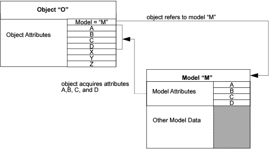
Key Concept—Model attributes are inherited by objects that refer to the model. They become part of the object’s attribute list.
A mechanism similar to that provided for model attributes allows object attributes to be passed upward in the modeling hierarchy. This mechanism is called attribute promotion. Promotion causes an object’s attribute to no longer have a value; instead, the attribute appears at the next level in the model. For example, for a module attribute in a node model, promotion moves the attribute into the node model’s attribute interface; this means that the attribute will be inherited by any node object in the network level that references the node model. In node objects in the network level, a promoted attribute is added to the attributes of the subnet that encompasses it. Attributes that promote all the way through the model hierarchy become attributes of the overall system model, or equivalently attributes of the simulation. These can be assigned values at simulation run time through a variety of mechanisms. It is then possible to iterate through a range of parameter values in different simulations to study the system as a function of the parameters.
Key Concept—Instead of having a value that is specified in advance, object attributes can be promoted. A promoted attribute moves up to the next level in the model hierarchy, allowing its specification to be performed there. Attributes that are promoted through the top of the hierarchy (top subnetwork) become attributes of the simulation.
Derived Models
In many cases, model developers need to customize a model’s interface without changing the model’s internal structure or behavior. Node and link model attribute interfaces can be modified using a mechanism called model derivation. Model derivation operates on an existing model and generates a new model that has different attribute interfaces. The resulting model is called a derived model, and the model from which it was created is called the parent model. A model that is derived from no other model (a very common case) is called a base model. All derived models have a unique base model that they refer to via one or more derivations.
The purpose of providing the derived model mechanism is to allow specialized interfaces to be developed without having to duplicate or recreate core functionality in a model. Because a parent model and its derived model are fundamentally the same in structure and behavior, specification of this information is shared. This provides economy of specification and enforces long-term consistency of these models as they are modified over time.
Key Concept—When a specialized version of a model is needed, a derived model can be created from it. The derived model shares the same structural and behavioral specification as its parent model, but parts of the parent’s interface may be altered. Successive derivations may be performed. A model that is not derived from any other is a base model.