Statistic Collection Mechanisms: Probes
In the case of most simulations, a large number of system variables and metrics are available for collection. Each module at the node level, as well as link at the network level is the source of a significant number of built-in local statistics, and in addition a simulation can generate large numbers of global and local user-defined statistics. However, in general, only a small subset of the available data is of interest to the simulation developer. Also, collecting all possible information would be prohibitive in terms of storage space and would negatively impact simulation speed. To address this problem, Modeler provides mechanisms to selectively specify which information should be collected as a simulation runs. These mechanisms are described in this section.
The flow of data into output files is controlled by a special object called a probe. Probe objects are not part of the model itself, and they do not affect the behavior of the model during simulation in any way. Instead, they play the role of a passive data collection device, “attached” to an object in the model that is capable of generating information in one of the forms described above. In the sense that it is passive, a probe is much like an ideal oscilloscope probe used in analyzing an electronic circuit. By decoupling probes from models, Modeler provides a powerful mechanism for quickly altering specification of data collection, without necessitating any changes to the model itself.
The purpose of a probe is to act as an enabler of output data that could potentially be stored in the simulation’s output files. Each source of data that is not explicitly probed is essentially “shut off”. Modeler takes the approach that output sources are off by default because the number of sources virtually always vastly outnumbers the number of sources of interest.
Probes can be specified using the Probe Editor, which allows the correspondence between probe objects and model objects to be established via a graphical selection. Any number of probes may be specified and the collection of probes is saved as a probe list. The probes of a probe list are applied as a group to a simulation model at the time that the simulation is executed. Multiple probe lists may be separately specified for the same model. They may then be applied to the model during distinct simulations, but only one probe list may be used for a given simulation run.
There are several different types of probes, corresponding to the different types of supported output and objects in Modeler. In broad terms, there are three types of probes: statistic probes, animation probes, and attribute probes. Within each of these categories there may be several additional varieties of probes. Each of these is described in this section and listed in the following table.
Table 117: Supported Probe Types
| Probe Type | Applications | Varieties |
|---|---|---|
| Statistic | Collect data of a numerical form generated either by built-in object statistics, or by user-defined local and global statistics. Can generate both output vectors and output scalars. | Node Link Path Global |
| Attribute | Capture values of object and simulation attributes as output scalars. These are viewed as “inputs” to the simulation model. | |
| Animation | Enable graphical animation commands to be issued by the simulation. Animations describe various aspects of system behavior. They can apply to particular objects, models, and statistics, or can be completely customized. | Automatic Custom Statistic |
Each probe is an object with a set of attributes that specify which output source it applies to, as well as various options concerning how to collect the data. The attributes vary for each type of probe. For details on the use of each attribute, see Chapter 4 “Probe Reference” on page 107.
Statistic Probes
Modeler supports local and global statistics. Local statistics are associated with particular objects, which the statistic probes must reference to collect data. The specific objects that support local statistics are nodes, links, and modules. Node statistics actually originate in modules or submodules within the nodes, but they are promoted to the node level by the node model specification (see Chapter 6 “Node Domain” on page 263 for more information on statistic promotion). This mechanism allows users of node models to access these statistics without having internal knowledge of the node model’s components. Node and module statistics are supported by the node statistic probe object, which provides attributes for specifying the physical object being probed, down to the submodule level if necessary. Node statistic probes support both built-in statistics of objects, as well as the user-defined statistics that are declared by process models. Link statistic probes provide access to pre-defined statistics that are computed for point-to-point and bus link objects. For complete information on the individual statistics that are pre-defined for each object, see Chapter 2 “Node Reference” on page 8 and Chapter 3 “Network Reference” on page 60.
Table 118: Objects that Generate Statistics
| Object Type | Statistics |
|---|---|
| Processor | Application-specific (defined by developer) |
| Queue Subqueue |
Application-specific (defined by developer), and statistics related to queue size, available queue space, overflow occurrences, queuing delays, etc. |
| Generator | Output levels, interarrival times, sizes of packets, etc. |
| Transmitter channel | Throughput, utilization, queue size |
| Receiver channel | Throughput, utilization, collisions, error rates |
| Link | Throughput, utilization, error rates; collisions |
Global statistics provide information that relates to the overall system. Many separate objects may contribute to one global statistic during a simulation. For example, every node in a network model may use the same global statistic to record the end-to-end delay experienced by the packets it receives. The result is one statistic for the network’s end-to-end delay performance. Global statistics are declared by process models and are supported by the global statistic probe object. Of course, no objects are referenced in a global statistic probe; only the name of the statistic is specified.
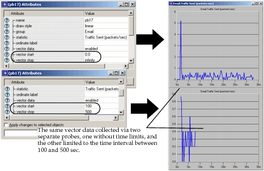
All statistic probes offer a set of common options that are specified via their attributes. Each probe can act as the source of both output vector and output scalar statistics, as specified by their “vector data” and “scalar data” toggle attributes. Both may be simultaneously enabled. If “vector data” is enabled, all of the values of the statistic are collected in an output vector in the simulation’s output file. The vector’s statistic collection can be restricted to a simulation time frame, as specified by the values of the “vector start” and “vector stop” attributes. This is useful to reduce the storage requirements for very dense statistics, particularly because only a portion of a statistic’s activity is usually of interest. Often, this period is at the end of the simulation, or after a particular event of interest (e.g., a component failure), to analyze transient behavior.
Figure 240: Limiting Vector Time-Spans with Probe Start and Stop Times
If a statistic probe’s scalar data attribute is enabled, the probe will generate one scalar value in the simulation’s output vector file at the end of the simulation. The scalar value is computed as a function of all of the statistic’s individual values over the course of the simulation according to a specified metric. As with output vector collection, the scalar statistics computation can be restricted to the values experienced by the statistic during a particular period. This period is specified using the “scalar start” and “scalar stop” attributes of the probe. The supported metrics are specified using the “scalar type” attribute and are listed in the following table.
Table 119: Scalar Types Supported by Probes
| Scalar Type | Description |
|---|---|
| last value | The value of the final update within the collection window |
| sample mean | The mean of the values of all the updates in the collection window (i.e., the sum of all the update values divided by the number of updates) |
| time average | The average value over time of the values generated during the collection window; this average is performed assuming a “sample-and-hold” behavior of the data set (i.e., each value is weighted by the amount of time separating it from the following update and the sum of all the weighted values is divided by the width of the collection window). For example, suppose you have a one-second bucket in which three values have been generated. The first one is generated at 0.1 seconds, the second at 0.2 seconds and the third at 0.9 seconds. Because the second one lasted for 0.7 seconds (0.9 - 0.2) it has a higher duration than the other two and is weighted more heavily in calculating the time average. |
| variance | The sample-oriented variance of all update values occurring in the collection window (i.e., the mean value of the square of the difference between the update values and their sample mean) |
| min value | The minimum value encountered during the collection window |
| max value | The maximum value encountered during the collection window |
In certain cases, statistics experience such frequent change during a simulation that collecting all of their values in output vector form becomes problematic. Specifically, one or more vectors may require a prohibitive amount of disk storage to be collected in their entirety. In addition, the frequent saving of the statistic may reduce the performance of the simulation, even though Modeler uses mechanisms to minimize this effect. In such cases, it may be desirable to reduce the size of the data that is being collected, even at the cost of a certain amount of accuracy or completeness. One mechanism that can be used is to limit the window of time over which collection is performed, as was described earlier in this section. Another approach, which can be applied separately or combined with windowing, is to reduce the values of the statistic at a specified rate to generate a less dense output vector. Statistic probes support “on-the-fly” processing of statistics, and particularly reduction of statistics, via their “capture mode” attribute. A probe’s capture mode specifies a method by which a statistic’s values can be modified as they are updated. The modified values are stored in the output file, rather than the “raw” values that are initially submitted to the probe. Four capture modes are supported, as listed in the following table.
Table 120: Statistic Capture Modes
| Mode | Details |
|---|---|
| all values | All updates to the statistic are recorded without modification. |
| sample | Records only certain statistic updates, and ignores others. Supports two modes: 1) retain every n_th update; or 2) retain an update every T seconds. |
| bucket | Considers a set of points called a “bucket” and records one value which is representative of the bucket. Buckets can be specified as time intervals or by the number of updates they contain. The retained value is computed as one of the following functions of the values in the bucket: sum/time, min value, max value, sample mean, time average, and count. This the default capture mode. |
| glitch removal | When multiple updates to a statistic occur at the same time, only the last update is retained. |
Figure 241: Comparison of Normal Mode and Bucket Mode
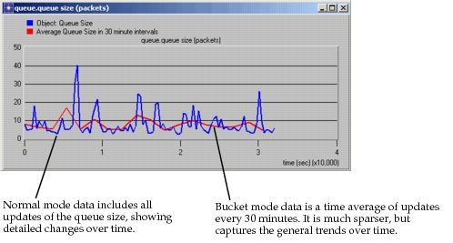
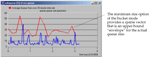
Depending on the statistic and the goals of the modeler, different capture modes or options of the capture mode may be more appropriate. Figure 241 shows the effect of using the bucket capture mode when collecting a quickly varying statistic, such as the size of a queue with roughly equal random arrival and departure rates. The bucket mode results are useful because they show the general trend of the statistic’s variations, even if they do not capture any of the rapid changes. However, because the changes are rapid, the time-averaged bucket mode output fails to show how high the queue size can get. With some statistics that can quickly rise and fall, this deficiency can be even more pronounced. If a buffer is being sized, for example, the peak values may be of interest. The result of using the bucket mode with a maximum value computation is shown in the following figure.
Figure 242: Comparison of Normal Mode and Bucket Mode with Maximum Value Option
Note: If the “scalar data” attribute for a probe is enabled, the “capture mode” attribute applies to the vector statistics used to derive the scalar statistic. Therefore, the capture mode can affect the final scalar data result.
Attribute Probes
Attributes specify characteristics of objects. Because they are part of the specification of a model, they can be viewed as “inputs” to the simulation. This is particularly clear when an attribute is promoted past the network level of the model and requires an assignment to be provided at the time of simulation execution. It is useful to introduce certain simulation inputs into the output files to facilitate studying the dependencies that exist between simulation outputs and inputs. For example, we may want to analyze how the throughput of a network varies as a function of the traffic load that is submitted. Or, we may be interested in the end-to-end delay of traffic as a function of the speed of the network’s transmission lines. In these cases, traffic load and transmission line speed are model inputs that we would vary over a series of simulation experiments. In each experiment we would record these inputs as well as the throughput and end-to-end delay. By recording the input and output quantities together we can establish the relationship that exists between them.
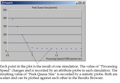
Because user-defined code can access the values of attributes and has the ability to also write values into the simulation output files, it is of course possible for process models to save attribute values in the simulation output files. Process models can also do computations that combine or otherwise process the values of multiple attributes. However, in cases where the values of numerical attributes are of interest without further processing, special probes called attribute probes can be used. Numerical attributes include the integer, double, toggle, and toggle data types. Each attribute probe applies to one object or simulation attribute and generates a corresponding scalar value in the output VECTOR file. The attribute probe has an attribute called “object” that allows it to refer to any object at the network or node level in the model. If a simulation attribute is declared by any of the process models in the system, an attribute probe can refer to it by leaving the “object” attribute blank. The following graph shows an example of a plot that can be obtained using an attribute probe for the independent variable (i.e., input), and a statistic probe for the dependent variable (i.e., output).
Figure 243: Scalar Plot Generated Using Output of Statistic and Attribute Probes
Animation Probes
Modeler provides a mechanism called an animation probe which is used to enable and configure the generation of animation information as a simulation runs. The basis for the use of animation probes is similar to that of statistic probes; namely that a very large amount of animation data could be collected in a typical simulation, while only a small part of it may actually be of interest. By specifically indicating which aspects or physical parts of a model should be animated, the flow of resulting information can be kept manageable.
Three types of animation probe objects, called automatic animation probes, custom animation probes, and statistic animation probes, may be placed in a simulation’s probe file to enable generation of animation data. Multiple probes of each type may coexist within the same probe file. Automatic animation probes and statistic animation probes both enable built-in animation capabilities of Riverbed models. They provide the simplest means of obtaining animations with a discrete event simulation, because no additional specifications are required within the model. Custom animation probes act as an enabling device for animation requests that are generated by user-defined processes. Custom animations provide flexibility to represent general information during an animation, but require programmatic specification by the model developer.
Automatic Animation Probes
Animation probes can be placed on objects in both the network and node domains. Depending on the type of object affected by the probe, different types of animations will result, as summarized in the table below. For complete descriptions of the functionality provided by each type of automatic animation, see Chapter 1 “Using the 2-D Animation Viewer” on page 1.
Table 121: Supported Forms of Automatic Animation
| Object Type | Automatic Animation Type |
|---|---|
| Subnetwork | Animation of packet flows over point-to-point and bus links present within the subnetwork. |
| Node (fixed, mobile, or satellite) | Animation of packet flows over packet streams within the node |
| Processor or queue | Animation of state-transitions of root-level process within selected module |
Each automatic animation probe includes attributes called “subnet”,” node”, and “module” used to specify the affected object. The “representation” attribute is then used to select the desired form of automatic animation. In addition, each probe includes attributes to restrict the simulation time window during which it will be active, and to control the positioning and dimensions of the resulting animation window. For a description of the automatic animation attributes, see Chapter 4 “Probe Reference” on page 107.
Custom Animation Probes
If automatic animations do not provide all of the functionality required by the model developer, Modeler allows the developer to create customized animations that are better-suited to, or more complete for particular applications. Customized animations are implemented using the Anim package Kernel Procedures (KPs) that called from process models or pipeline stages. These procedures provide general drawing and animation capabilities as well as functions related specifically to displaying models. See Chapter 2 “Animation Package” on page 1for complete specifications.
Because animation can significantly degrade simulation performance, it is important to be able to selectively enable its generation. In particular, during long simulation runs, or sequences of simulation runs, animation is usually disabled entirely. Because custom animation is generated by user-developed logic, it is possible for developers to incorporate their own animation control mechanisms. In general, such a mechanism could be based on the use of object or environment attributes, queried using the KPs of the Ima package. Based on the values of these attributes, animation code could be conditionally executed.
Modeler provides a built-in mechanism for selectively enabling animation, called custom animation probes. Just like an automatic animation probe, a custom animation probe is associated with an object from the network or node domain. However, rather than resulting in the generation of a standard form of animation, a custom animation probe serves as an enabling agent for the animation directives that are executed within the context of the probed object. In other words, by default, calls to animation-related Kernel Procedures are ignored, unless an appropriate custom animation probe is defined to enable their actions.
The context of a custom animation probe, or the scope of animation directives that it can enable, depends upon the type of object to which it is applied. Ultimately, the source of custom animation directives must be either process model logic or transceiver pipeline stage logic, because these are the interfaces supporting the integration of user-developed code. For a processor or queue to be the subject of a custom animation probe implies that animation directives executed by any of the processes contained within it can make use of the probe. This extends to the procedures of a process’ function block and to procedures defined in external files, while they are executed in the context of the probed module. Similarly, if a transceiver is the subject of a custom animation probe, then animation directives issued from within associated pipeline stages, including indirectly called procedures, are affected by the probe. The following table lists the scope of custom animation probes for each supported object type.
Table 122: Scope of Custom Animation Probes
| Type of Probed Object | Enabled Sources of Animation Directives |
|---|---|
| Subnetwork | All processes executing within modules contained at any level of depth; in addition, all pipeline stages associated with transceiver modules or with links contained at any level of depth. |
| Node | All processes executing within any processor or queue contained within the node; in addition all pipeline stages associated with transmitter or receiver modules within the node. |
| Processor or Queue | All processes executing within the processor or queue. |
In the case of transceiver pipeline stages, there is a well-defined association with either the transmitter that acts as the source, or the receiver that acts as the destination during a pipeline execution. The following table summarizes this association for the purposes of determining where to place animation probes.
Table 123: Transceiver Associations for Pipeline Stages
| Pipeline Type | Transmitter-Associated Stages | Receiver- Associated Stages |
|---|---|---|
| Point-to-Point | transmission delay, propagation delay |
error allocation, error correction |
| Bus | transmission delay, closure, propagation delay |
collision, error allocation, error correction |
Custom animation probes have a set of attributes that is essentially the same as that of automatic animation probes: attributes specifying the probed object, a time-window of effectiveness, and the geometric properties of the display window. In addition, an attribute called “label” can be used to specialize the applicability of the probe. User-defined code can determine if a probe with a particular label exists, and if so, which animation viewer (i.e., animation window) is associated with that probe. The code can then enable appropriate animation requests and direct them to the required windows. The label also serves as a rendezvous mechanism, allowing different processes and pipeline stages to obtain the same animation viewer ID and coordinate their activities within the same window. The meaning of probe labels are user-defined, but the Simulation Kernel supports this feature with the KP op_anim_lprobe_anvid(), which converts a label to an animation viewer ID. For more information on the use of custom animation labels, see Chapter 2 “Animation Package” on page 1. For more information on the “label” attribute, see Chapter 4 “Probe Reference” on page 107.
Statistic Animation Probes
Statistic animation provides the capability to dynamically view output vector statistics as they evolve over the course of a simulation. The graph that is presented in a statistic animation appears in an “analysis panel” that is similar to the one displayed in the Results Browser. However, it adjusts dynamically by rescaling and scrolling to accommodate the changing bounds of the output vector as updated values are received from the simulation. Each statistic animation probe uses the “scrolling” attribute to specify if a fixed-width time window of the statistic should be displayed, or if instead, the entire history of the vector should be shown by continually expanding the time axis as time progresses.
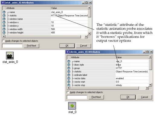
Statistic animation probes can only work in association with other statistic probes. In other words, a statistic animation can only be provided for a statistic that is already probed via a node, link, or global statistic probe. The statistic animation probe uses its “statistic” attribute to establish an association with a statistic probe. The value of this attribute must match the full hierarchical name of the statistic as specified in the statistic probe (see the example in Figure 244), or the “ordinate label” of the statistic probe, if one has been specified. Options of the corresponding statistic probe, such as start and stop times, and capture mode, automatically apply to the statistic animation probe. The final graph that is obtained at the end of a statistic animation is therefore identical to the output vector that results from the statistic probe.
Figure 244: Association of Statistic and Statistic-Animation Probes
Note: The “window name” attribute must have a unique value for each animation probe. You cannot view multiple animations in one window.