Estimating the Benefit of Parallel Simulation
The gain in performance from parallel execution of model code depends on the distribution of events in time and the computational intensity of those events. Models that benefit the most from parallel event execution have the following characteristics:
- Events that are “expensive” in terms of computation time
- A substantial density of events that occur in the same parallel execution window
- Events that occur in different parts of the network
Determining how fast a simulation will run in parallel is not a trivial task. However, both the sequential and parallel development kernels can produce event instrumentation reports that can be used to estimate the expected gain in performance.
The base metric for a performance estimate is the average number of events in each parallel execution window (also called a cell). In the worst case, simulations with an average of one event per window will realize no performance gains from the parallel kernel because no events are processed in parallel. On the other hand, simulations with high average event counts per window can benefit from parallel execution. However, that number alone does not guarantee increased performance because multiple events in a window might be “chained”. That is, one event in a window generates subsequent events in the same window, but that event must finish executing before the subsequent events can begin executing. This happens relatively frequently in simulations where data is passed between different layers of node models and no time delay is being modeled between layers.
Increasing the “parallel_sim.event_execution_time_window” preference or scaling up the model size make it more likely that multiple events will occur in the same window. Therefore, even if the initial study shows that a network model is unlikely to benefit from parallel execution, the situation may change for a larger model.
The question of what values are acceptable for “parallel_sim.event_execution_time_window” must be considered carefully. For example, most packet transmission protocols use a back off or retransmission interval; consequently, the “parallel_sim.event_execution_time_window” should never be bigger than the mean interval value. If your model has a 0.1-second timeout, the window must be smaller than 0.1. Making the window too large will produce different output statistics or event counts.
Parallel Speedup Report
The sequential development simulation kernel can generate a parallel speedup report that estimates the highest theoretical speed improvement that can be achieved by running a simulation on a multiprocessor system. This report can be generated without making existing models parallel-safe. Therefore, because some protocols and models may not have enough inherent parallelism to justify the model development resources needed to make them parallel-safe, the parallel speedup report can be a valuable measure of whether a model can benefit from parallel processing before any time is spent making models parallel-safe. It is a first-cut determinant of possible benefits.
To generate the report, use the ‑verbose_parallel_speedup_report command line option to a development simulation kernel. A speedup report similar to the one in the following figure is produced at the end of the simulation.
Figure 252: Parallel Speedup Report
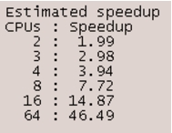
The estimated speedup in the report is the highest theoretical speedup, which can be achieved only by a model that can run all code in parallel with no contention caused by forced serialization. Because there is always some shared-data serialization in any model, the real speedup realized in the parallel kernel will never attain the theoretical maximum.
The following command-line options enable more detailed and advanced instrumentations that can be performed by both sequential and parallel development simulation kernels:
-verbose_cell_size_report-verbose_event_timing_report
Cell Size Report
The -verbose_cell_size_report option shows the distribution of event counts in time windows at two points in time:
- when the first event in a window started executing (the “in” columns)
- when all the events in a window finished executing (the “out” columns)
The parallel kernel also reports the events processed in parallel versus the events processed sequentially. This allows you to see how many events the kernel processed in parallel.
When the “verbose_cell_size_report” preference is set to TRUE, the sequential kernel produces the following output with each simulation progress update (generated according to the “update_interval” preference for number of events):
Figure 253: Simulation Progress Update Generated by the Sequential Kernel
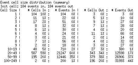
The table in Figure 253 represents a histogram of event distribution among cells (time windows). This table can be used to analyze the potential for parallel simulation speed improvement: simulations with more cells that start “heavy” (a lot of “in” events) are likely to benefit more from execution in the parallel kernel. The table columns present the following information:
- Cell Size – number of events in a cell.
-
Cells In – number and percentage of cells that start with the given size.
-
Events In – number and percentage of events falling in cells of the given starting size.
-
Cells Out – number and percentage of cells that end with the given size.
-
Events Out – number and percentage of events falling in cells of the given ending size.
For example, there are 11 cells that start with a size of 2, for a total of 22 events. Only 5 cells ends with a size of 2, for a total of 10 events.
Cells can contain more events at their end than at their start because additional events can be scheduled during a cell for execution later in that cell. Thus, a given cell might be counted in one row of the # Cells In column, and in a lower row (greater cell size) in the # Cells Out column.
The table in Figure 253 also provides a clue to the useful size of the time window. If the “Out” columns are the same (or similar to) the “In” columns, the cell duration as set in “parallel_sim.event_execution_time_window” is a good one for parallel execution. In general, you can increase the time window until the “In” and “Out” columns become noticably different.
Figure 254: Distribution of Initial and Final Cell Size During Sequential Processing
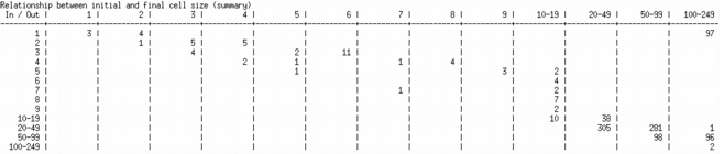
The table in Figure 254 shows the relationship between the initial number of events upon cell entry and the total number of events processed in that cell. The vertical axis represents the initial cell size (number of scheduled events at the start of the time window) and the horizontal axis represents the final cell size (number of events processed). For example, the first row indicates that, of the cells that had one event upon entry:
- three cells had just that entry event processed
- four cells had one additional event scheduled and processed (final size of 2 events)
- 97 cells had between 100 and 249 total events processed
Simulations for which the bulk of values appear in the lower-right corner of the table are likely to gain speed in the parallel kernel, because there are lots of cells with lots of events in each. When most of the events are in this category, you can infer that
- small cells don’t grow, so that parallelization will be accurate
- there are many big cells, so that parallelization will be fast
Events that are too close together to safely parallelize appear in the upper-right corner of this table (this includes the first cell in the simulation, containing the BEGINSIM interrupt and the immediate events derived from it). Events that are too far apart to parallelize (based on the current duration of the time window) appear in the upper-left corner. The lower-left corner is always empty.
The parallel kernel also provides information about the distribution of MT-safe (parallel) and unsafe (sequential) events executed in each window, as shown in Figure 255.
Figure 255: Distribution of Parallel and Sequential Events Executed by the Parallel Kernel
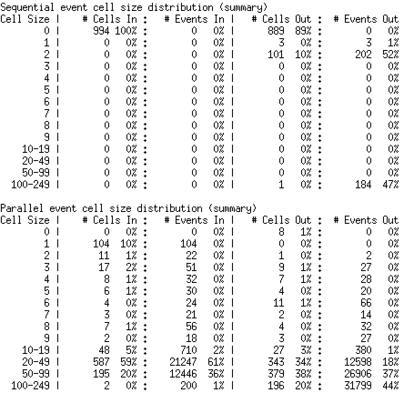
For the “In” statistic, all events that are tagged as capable of being processed in parallel are reported as “mt-in” events. However, if those events were the only events in a window at the time they were executed, they are counted as sequential for the output statistic. In this example, although all events are mt-safe upon entry—100 percent of windows had 0 sequential events upon entry—some events were still processed sequentially, as you can see in the sequential events out column. Fortunately, the bulk of windows (more than 81 percent) had 50 or more events processed in parallel.
Event Timing Report
The -verbose_event_timing_report option produces a report that provides event “weight” distribution details. For a given number of events in a window, it collects the average event processing rate. This information can be useful for detecting cases in which windows with a small number of events take the bulk of the real simulation time to process. This situation can limit the speed gains of parallel simulation because the total real-time savings from processing lightweight events in parallel might be insignificant compared to the real time spent in sequential processing. Remember that a high processing rate means inexpensive events and a low rate suggests events that are computationally expensive.
Figure 256: Event Processing Rate Report
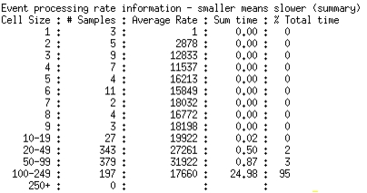
In this report, the # Samples column reports an internal measure roughly proportional to the number of events in cells of each size. As with earlier tables, large numbers at the bottom of the table are evidence in favor of parallel execution.
Summary
In summary, observe that:
- Not all models will benefit from parallel execution.
- The sequential development kernel provides reports that might help you decide if a model is likely to benefit from parallel execution.
- To analyze the potential for parallel execution, increase the time window up to the smallest protocol-specific time in the network (such as backoff or timeout interval) or until simulation results (such as number of events) change. Then check the Parallel Speedup report.
- Before making changes to existing model code, examine the report output to determine whether models are candidates for parallel execution. Larger numbers at the bottom of the report tables indicate good candidates.
- Using the same reports in the parallel kernel might help identify parallel model execution bottlenecks.
- Collecting information for these reports slows the simulation (as is common for any profiling utility).