Interfaces Menu Operations
This section contains descriptions and procedures for using the operations available from the Interfaces menu in the Process Editor. The items that appear on this menu are described below in alphabetical order.
- Interrupt Code Map
- Global Attributes
- Global Statistics
- Local Statistics
- Model Attributes
- ODB Labels
- Parallel Execution Support
- Process Interfaces
Interrupt Code Map
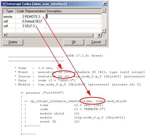
This operation lets you assign text strings that will be printed along with interrupt codes when they appear in ODB event banners and traces of various op_intrpt_schedule_ KPs. This mapping makes the interrupt codes easier to interpret during debugging. You can map codes for procedure call, process, remote, and self interrupts.
Note: These interrupt codes are the user-defined codes specified when scheduling an interrupt and returned by the op_intrpt_code() KP.
Figure 195: Interrupt Code Dialog Box and Sample ODB Output
Global Attributes
This operation allows you to define new global attributes and to edit or delete existing ones. Global attributes are not associated with any particular object, but are scoped globally to the simulation as a whole. Typically, global attributes are needed by an entire class of objects in a simulation, such as all of the processes of a particular type. These processes share the global attribute and so are guaranteed to agree on its value (as opposed to process model attributes, which provide each process model instance with its own independent value).
A process can query global attributes by using the KP op_ima_sim_attr_get(). Declaration of the global attribute in the process model supports several important mechanisms of other tools. In the Probe Editor, attribute probes can be set to collect the values of global attributes as scalar values. In the Simulation Sequence Editor, declared global attributes can be assigned values prior to executing simulations, thus avoiding the need to obtain the value dynamically as the process's request is encountered by the Simulation Kernel.
For more information about global simulation attributes, see
Global Statistics
This operation declares named global statistics that can be recorded during simulation and viewed as results. Global statistics are scoped to the simulation as a whole, in contrast to local statistics, which are scoped to a particular queue or processor. In other words, multiple processes, as well as pipeline stages, all at different locations in the model's system, can contribute to the same shared statistic. This is done by referring to the statistic by name and obtaining a statistic handle (see "Statistic Handles" on page 4 for more information). Global statistics cannot be used as the sources of statistic wires.
When you choose Interfaces > Global Statistics, the Declare Global Statistics dialog box appears (Figure 196). In this dialog box, you can create a new global statistic, delete an existing statistic, or modify some aspects of a statistic. To sort the table, click in a heading cell. Repeated clicks toggle the sort order.
Note: Advanced users might find it easier to declare large numbers of global statistics by editing a list manually and importing into the table. See Editing Local and Global Statistic Declarations for details.
Figure 196: Declare Global Statistics Dialog Box
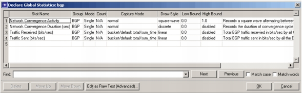
The following table lists the fields in the Declare Global Statistics dialog box.
Table 102: Declare Global Statistics Dialog Box—Fields
| Name | Description |
|---|---|
| Stat Name | Name of the statistic defined by the process model. |
| Group | Group the statistic belongs to. This group is used to organize the statistic in the hierarchy shown in the statistic browser. |
| Mode | Number of dimensions. A single-mode statistic generates only one independent series of values over time. A dimensioned-mode statistic actually represents a set, or array, of single-mode statistics, each independently managed and separately usable for probes and statistic wires. Each of the individual statistics in a dimensioned statistic shares the same base name, but is distinguished by its index in the statistic array. This scheme is useful when managing large quantities of similarly defined statistics. For example, the performance statistics of a switch, with respect to each of eight outgoing links, could be declared using dimensioned statistics instead of individually declaring each one. This approach is more scalable, allowing the process model to more easily track growth in the node model simply by increasing the dimension of the statistic array. |
| Count | The number of elements in a dimensioned statistic. Similar to the dimension of an array. |
| Capture Mode | Default capture mode for the statistic. See "Project Editor" on page 89 for details about capture modes. |
| Draw Style | Default draw style for the statistic. |
| Low Bound | The lowest ordinate shown on a graph when the statistic is plotted. The low and high bounds are considered when drawing graphs, although the bounds are not absolute limits. Most statistics do not collect negative values, so you can usually set this value to 0. Built-in statistics have a low bound of 0. |
| High Bound | The highest ordinate shown on a graph when the statistic is plotted, as long as the actual results are less than the high bound value. If a value collected for the statistic is higher than the high bound you set, the vertical axis will be expanded so the highest data point can be graphed correctly. |
| Description | Brief description of the statistic. Left-click to display the full description in a text edit pad. |
For more information about global statistics, see
Local Statistics
This operation declares named statistics that can act as sources of statistic wires at the node level, as well as node statistic probes defined in the Probe Editor. Local statistics are scoped to the queue or process module in which a process operates. In other words, each separate instance of the process model can individually maintain a local statistic with the same name. These statistics vary independently over time, can be separately probed, and can be used to feed statistic wires.
When you choose Interfaces > Local Statistics, the Declare Local Statistics dialog box appears (Figure 197). In this dialog box, you can create a new local statistic, delete an existing statistic, or modify some aspects of a statistic. To sort the table, click in a heading cell. Repeated clicks toggle the sort order.
Note: Advanced users might find it easier to declare large numbers of global statistics by editing a list manually and importing into the table. See Editing Local and Global Statistic Declarations for details.
Figure 197: Declare Local Statistics Dialog Box
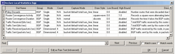
The fields in this table are the same as for the Declare Global Statistics dialog box, as listed in Table 102.
For more information about local statistics, see
Model Attributes
This operation allows you to define new process model attributes and to edit or delete existing ones.
Process model attributes are essentially "parameters" of the model, allowing users of the model to control its behavior in predefined ways. Process model attributes are automatically promoted to the node level, where they appear as attributes of processor and queue modules.
An important function of process model attributes is to generalize the applicability of a process model. Specifically, rather than embed a fixed characteristic into a process model (such as a "hardwired constant"), this same characteristic can instead be represented by a process model attribute. Each instance of the process model, or process, learns of its particular attribute assignment when the simulation begins and adjusts its configuration or behavior appropriately. In this way, the process model has achieved a greater degree of reusability by supporting a broader set of applications. The alternative is to create many process models that are nearly-identical except for a small number of built-in characteristics. This is a less desirable approach because it entails maintaining a larger implementation and requires continually duplicating process models as slight variations become necessary. Furthermore, by using process model attributes to parameterize behavior, simulation sequences can automatically sequence through different scenarios simply by changing attribute values.
For more information about process model attributes, see "Process Domain" on page 165.
ODB Labels
This operation lets you associate descriptions with any labels used in a process model. This information can be displayed in the Simulation Debugger. (See the ODB command "lmap" on page 117.) The labels and descriptions you define here should reflect the labels used in process model code. However, there is no enforcement on the validity of the defined labels, nor do they affect compilation of the process model or its use in ODB.
Parallel Execution Support
This submenu lets you specify whether or not the code in the current process model is MT safe (and thus whether the events executed by the process model can be executed in parallel).
The choices are:
- Support Parallel Execution – The process model is MT safe and can be run in parallel.
- Does Not Support Parallel Execution – The process model is MT unsafe and is always run sequentially.
- Model Safety Has Not Been Studied – MT safety is unknown. Whether the code will be run in parallel or sequential mode is determined by the "parallel_sim.unknown_process_mt_safety_handling" preference.
WARNING: Do not select the Support Parallel Execution option unless the process model code is MT safe, as described in "Making Models Parallel-Safe" on page 413.
Process Interfaces
This operation allows you to set values for and specify the behavior of the built-in attributes of queues and processors. The functions supported by this operation are a subset of those supported by the node model interface for built-in attributes of node objects. See "Node Interfaces" on page 461 for a description of these functions.
Figure 198: Process Interfaces Dialog Box
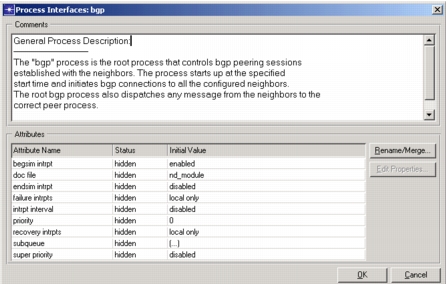
A process model's attribute interface is somewhat simpler than that of a node model because, unlike a node model, a process model contains no objects that promote attributes to the next modeling domain. The only attributes that a process model promotes to the node level are process model attributes. However, process model attributes are not affected by the process model attribute interface, just as node model attributes are managed separately from the node model attribute interface.
The process model attribute interface therefore applies only to control of built-in attributes of queues and processors. This mechanism is useful to simplify the attribute lists of queues and processors and to enforce particular attribute settings that the process model relies on. For example, a process model implementing a statistic collection process may rely on the receipt of an end simulation interrupt. The process model developer can guarantee that a processor module will provide this service by enabling and hiding the "endsim intrpt" attribute of the processor via the process model attribute interface. By hiding the attribute, the process model developer prevents its value from being changed at the node level.
Not all built-in attributes of queues and processors can be controlled in this way. For more information about specific built-in attributes that can be affected by lower-level model attribute interfaces, see "Modeling Concepts".