Process Model Operation
Node objects are used to represent devices that can be connected together to form networks. Devices may range from simple traffic sources to complex switches or computers running multiple applications. Nodes are created as instances of node models, meaning that a node model is the blueprint for all of the individual nodes of a particular type. Node models are defined as a collection of modules representing distinct functional areas of the node. Certain modules are limited in the types of behavior they can represent; for example, the various transmitters and receivers represent interfaces to links defined in the network domain.
Three types of modules—called processors, queues, and esys modules—support fully general behavioral modeling. These modules offer essentially the same capabilities with regard to their general behavior and most of their physical resources. However, two of these provide additional capabilities:
- Queue modules provide special support for organized packet storage by enabling users to define internal subqueues in which packets can be inserted and sorted, and from which packets can be extracted according to a general, user-defined method.
- Esys modules provide queueing abilities and the ability to specify an ESD model for cosimulation.
For the most part, esys modules, queues, and processors can be treated identically because they rely on the same process modeling technology to represent their behavior. Therefore, in this manual the term QP is used to represent these modules.
Process Environment
Individual processes or groups of processes are defined to implement a particular task when placed within a QP. A process is an instance of a process model defined with the Process Editor. In other words, each process model may be assigned to many QPs within one system. All individual process instances are defined to have similar characteristics but may operate in different environments.
Process models do one of two functions, depending on the QP. A process model typically represents a behavioral model of a process, as explained below. Esys modules, however, can also use a process model to handle interaction with an external system. Effectively, the process model becomes part of an interface between Modeler and the external system during a cosimulation. This section describes in general terms the context in which processes do their functions.
Interrupt-Driven Execution
Like all other subsystems in Modeler models, processes are driven by events. When an event is actually delivered to a process, it is termed an interrupt, as defined in Chapter 4 “Modeling Framework” on page 80; the process is said to be interrupted which means that it is invoked to allow it to take some action in response to the interrupt.
The reasons for which a process may be interrupted vary widely from process to process, and most processes themselves expect several types of interrupts signifying different conditions to which they must respond. Therefore, one of the first actions that is generally taken by a process upon being interrupted is to determine what type of interrupt has occurred. Subsequently, more detailed attributes of the interrupt might also need to be analyzed. Depending on the interrupt type, these attributes might be the input stream or statistic, the esys interface that has a new value, the source module that caused the interrupt, or possibly application-specific information contained in an Interface Control Information (ICI). Chapter 4 “Modeling Framework” on page 80 has a detailed description of interrupt processing.
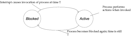
A process follows an alternating cycle of invocation and rest periods. Invocations may occur on an arbitrary basis depending on the timing of externally and internally generated events. A process always begins the simulation in a resting mode, waiting to be invoked; a process that is waiting in this conditions is said to be blocked. Invocation allows a process to resume execution and to do new actions. After these actions are completed, the process must again block, returning control to the Simulation Kernel so that other events in the system may be executed. Because these subsequent events may be scheduled for arbitrarily near future times, and even for the same time as the current event itself, the invocation must occur without allowing any time to elapse. In other words, the simulation time observed (e.g. by calling the KP op_sim_time()) at the start and at the end of an event, must always be identical. Note that this requirement does not imply that processes cannot model actions that consume time; only that modeling such actions can sometimes require multiple events. The requirement for zero-delay execution of events and techniques for delay modeling are explained in detail in Chapter 4 “Modeling Framework” on page 80. The following figure depicts the alternating sequence of blocking, invocation, activity, and back to blocking.
Figure 90: Process Blocking/Activity Cycle
Dynamic Processes
At the moment when a simulation begins, each QP hosts only one process that is automatically created by the Simulation Kernel. This process, termed the root process, is an instance of the process model designated in the QPs “process model” attribute. The root process model can be designed to manage even very complex sets of tasks, and so depending on the application, the root process may be sufficient to provide the QP module with its intended functionality. However, in many modeling situations, it is possible to take advantage of the capability of a QP to host multiple processes to improve the modularity and reduce the complexity of a design.
New processes become associated with a QP module when the processes that are already present within it request their creation via the KP op_pro_create(). One QP might be the host to many processes that cooperate to implement its function within the surrounding node model. Processes that are created by other processes (as opposed to the root processes created by the Kernel) are referred to as dynamic processes. There are two principal cases in which a QP generally makes use of dynamic processes:
- At least part of the QPs functionality requires it to manage tasks that are generated on a dynamic basis (when their exact timing or number are not known in advance). In such cases, a new process can be generated to correspond to each task as it arises. The process can then be destroyed when the task is complete. Because there is no upper limit on the number of processes allowed in a QP, any number of concurrent tasks can be handled this way. A typical example of this of application of dynamic processes is the implementation of a circuit-oriented protocol such as X.25, where new circuits are opened and closed based on incoming requests whose patterns are unpredictable. Each circuit can be managed by an independent process, and all circuits can flow through the same QP module, allowing one module to represent the functionality of the protocol within the node.
- The activities of the QP are conveniently represented as multiple asynchronously running processes. The required processes may all be created when the QP configures in the beginning of the simulation and may remain the same throughout the simulation afterwards, each process implementing a subset of the overall QPs functionality and perhaps cooperating with other processes to support their activities as well. Generally this approach is used when a QP is required to manage several tasks in parallel, each of which is substantially independent of the others.
Process Hierarchy
Because dynamic processes are always created by other processes, the root process must be involved in originating them. The first generation dynamic processes (i.e., those generated by the root) may then in turn create new processes, which would be referred to as second generation. With respect to a process that creates it, a dynamic process is referred to as a child process; conversely, the creating process is referred to as the parent process. Because all processes have the capability to create others, the processes within a QP form a tree structure with the branches representing parent-to-child relationships. The root process is the ultimate “grandparent” of all processes.
Figure 91: Typical Process Hierarchy within a QP
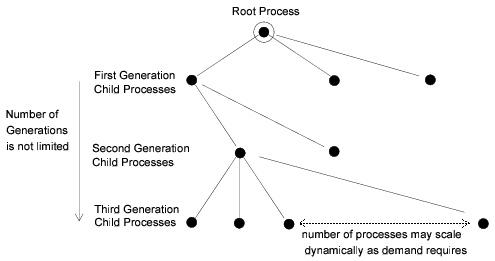
Because processes can be destroyed as well as created, the process hierarchy may shrink as well as grow. In addition, there is no requirement that a process’ children must all be destroyed before it can itself be destroyed; therefore “holes” may appear at certain levels within in the process hierarchy, corresponding to the fact that certain processes have no active parent processes. Note however that the root process plays a special role in handling interrupts for each QP, and that it is the only process that may not be destroyed. The role of the root process is addressed in a subsequent section on interrupt steering.
Note that a process is capable of creating child processes of any type (i.e., based on any process model), including its own or the type of its parents; however, a complete list of child process models that it intends to instantiate must be declared prior to simulation as part of the process model definition. Attempting to create a process based on a process model that is not declared may result in an error during simulation. The Process Editor provides an operation called Declare Child Process Models that supports menu-based editing of the potential child process list. See “System Menus” on page 29 for more information on this operation.
Promoted attributes of a child process are promoted along with those of the parent process, and therefore appear in the attribute lists of queues and processors at the node level. The child process’s attributes are prefixed with the name of the process model to differentiate them from other similarly-named attributes.
Shared Memory Architecture
When a QP relies on multiple processes to implement its functionality, these processes often require some form of communication between them to cooperate in managing the QPs tasks. The Simulation Kernel therefore provides three communication mechanisms that allow multiple processes to share information. These mechanisms may be used individually or combined.
-
QP-level shared memory: This form of memory, also referred to as module memory, allows all process in a QPs process hierarchy to communicate information to each other by placing this information in a common area. Each QP maintains one memory address that processes can assign or obtain by calling the Kernel Procedures op_pro_modmem_install() and op_pro_modmem_access(). The various processes that use this mechanism must agree on the format of the data that is pointed to by the shared memory pointer. In general this is done by defining a data structure that can be referenced by all processes. To ensure that all processes use a consistent form of the data structure, even when it is changed, the definition should be kept in an external definition file that is included in each process’ header block; in the C language, definitions files are named with a “
.h” suffix.Figure 92: Coordination of QP-Level Shared Memory
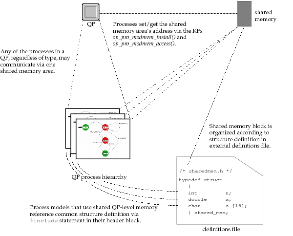
Initially, the Simulation Kernel provides no shared memory for a QP (the Kernel Procedure op_pro_modmem_access() returns a NIL value to indicate that this is the case); it is up to the processes within the QP to decide how much memory is necessary and when it should become available. The processes are therefore responsible for allocating the block of shared memory, after which it can be installed by calling op_pro_modmem_install(). Memory allocation is generally performed by calling op_prg_mem_alloc().
It is possible for a shared memory block that has been installed to be replaced by another. The KP that supports installation simply allows a new memory address to take the place of the existing one, without protecting against loss of the data that was previously installed. Therefore process architectures that do multiple installations are responsible for any required memory deallocation.
In practice, a shared memory block is usually installed only once and this installation is performed by the root process when it is invoked for the first time. This allows other processes in the hierarchy to simply assume that the memory is available. After QP-level shared memory has been installed, processes may communicate information to each other by writing data into the common memory space. This is generally done by assigning values to the members of the installed data structure. Other processes then examine the contents of the data structure and make use of this information as required. Communication between the processes using module memory can be on an active basis or on a passive basis. Active communication involves modifying the shared memory contents and then invoking the process that is to receive the new information (invocations between processes are performed with the KP op_pro_invoke()). Passive communication simply involves modifying the shared memory contents, but relies on the destination process to autonomously examine the shared memory, perhaps at a later simulation time.
-
Parent-to-child shared memory: in many cases, the communication that must take place within a QPs process hierarchy is between processes and their parents. This is due to the fact that child processes are often created to handle parts of a parent process’ work and that results must be reported back to the parent. The Simulation Kernel provides specific support for this type of communication by allowing a private shared memory area to be set up at the time that a child process is created. Other processes do not have access to the memory, although they may reserve their own parent-to-child memory. The Kernel maintains an independent shared memory block for each parent-child pair in the system.
Figure 93: Parent-to-Child Shared Memory Organization
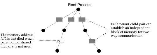
As is the case with all inter-process memory mechanisms, parent-to-child memory is optional and may exist only between certain parent-child pairs. Unlike QP-level shared memory, however, parent-to-child memory may only be installed once for each parent-child pair, when the child process is created with the Kernel Procedure op_pro_create(). Replacement of the memory block is not possible, although it may be deallocated when it is no longer necessary. A process may obtain the address of the memory that it shares with its parent process by calling the KP op_pro_parmem_access(). However, because a parent process might have many child processes, and because it must supply the addresses of parent-child shared memory, it is responsible for keeping its own records of such addresses (e.g., by storing them in state variables).
In general, parent-to-child shared memory is allocated by calling the KP op_prg_mem_alloc(). The format of the shared memory is transparent to the Simulation Kernel, which only manages the memory block’s address. However, as in the case of QP-level shared memory, the parent and child processes must agree on the memory format and this is usually accomplished by referencing a common definition of a C or C++ data-structure to allocate and access the shared memory. After the shared memory block is established (i.e., when the child process is created), both the parent and the child may communicate information with each other by modifying and/or examining the memory contents. If applicable, they may choose to actively invoke each other to provide notification of changes to the shared memory area by calling the Kernel Procedure op_pro_invoke().
-
Argument memory: communication between processes is often required at the time that one process transfers control to another by invoking it with the Kernel Procedure op_pro_invoke(). To support this type of information passing, op_pro_invoke() accepts a general memory address as an argument and makes this address available to the invoked process. As with the other two memory mechanisms, the memory address points to a block of memory whose format is user-defined and the two processes must be designed to agree on how its contents are organized. The invoked process obtains the memory address by calling the KP op_pro_argmem_access(). It may then use the memory to obtain parameters that affect its behavior, and/or modify the memory to return status information to the process that invoked it. Note that unlike the other two memory mechanisms, argument memory is not persistent. This means that each new invocation of a process requires that an argument memory address be passed again, even if it is the same as the address supplied for a previous invocation between the same two processes.
Each of the mechanisms described above supports communication of information via an abstract data object in the sense that the Simulation Kernel does have knowledge of the structure or contents of the shared information. The memory address is manipulated as a general pointer and the process logic is required to cast or coerce the type of the pointer so that it becomes a pointer to an appropriate data structure, as agreed upon by the various communicating processes. Also note that each memory mechanism supports two-way communication of information because all processes that have access to a memory block may both insert and extract information from it. For more information about process shared memory mechanisms, see “Process Package” on page 1.
Operations on Dynamic Processes
All interactions between dynamic processes are performed via the Kernel Procedures (KPs) of the Process package. In addition, several KPs in the Interrupt package provide capabilities that indirectly affect the operation of processes. Complete information on these procedures is presented in the “Discrete Event Simulation API”. The general capabilities provided by these KPs and related process model design issues are reviewed in this section.
As mentioned earlier, only one process initially exists in each QP, and this is the root process specified in the QPs “process model” attribute. Additional processes may be spawned when the root process (and subsequently other processes) calls the KP op_pro_create(). When a process model is created, it is implicitly incorporated into the process hierarchy of the process that created it. There is no way to create a process in another QP than that of the current process.
To create a child process, its process model should be declared in the specification of at least one of the existing processes. Declaration is performed via the “declare child process models” operation in the Process Editor. While it is sufficient for the created process’ model to be declared in the models of any of the QPs processes, it is generally a good practice of modular design to declare as part of each process model, the names of all the processes that it is capable of creating. This way, each process is responsible only for declaring the process that it directly creates, and new process models can always be included in a process hierarchy without concern for their own potential use of dynamic process creation.
When a process is created, a special data item called a process handle is returned by op_pro_create(). The data type used to declare a process handle variable is Prohandle. Process handles uniquely identify a process, not only within a process hierarchy, but within the entire modeled system (i.e., across all QPs). Process handles are required by most KPs in the Process package and so they are commonly used by models that employ dynamic processes. Generally, a process uses process handles declared as state variables to retain access to the process handles that it obtains when it creates child processes. This allows it to do fundamental operations on its children later, such as invocation or destruction. Process handles may also be obtained by several other KPs including op_pro_self(), op_pro_parent(), and op_pro_root().
Two other forms of process identification are provided, but neither is necessary to use the Kernel Procedures that affect processes. Process IDs are unique integer numbers that are automatically assigned to processes when they are created. A process ID can never be changed, nor can it recur within the same simulation. Process IDs are used to represent processes in informative output issued by the debugger included with Modeler or by user-developed reporting statements. A process’ ID can be obtained by calling the KP op_pro_id(). A process tag is a user-supplied string that may be assigned to a process at any time. The content of the string is transparent to the Simulation Kernel and is currently used only to identify processes or report special information about them as part of the output of the ODB command promap.
Certain dynamic processes are created to manage activities whose time-spans are limited, and their usefulness therefore expires when such activities complete. To avoid buildup of inactive processes, all dynamic processes (e.g., all processes but the root) may be removed from their QPs process hierarchy by application of the KP op_pro_destroy(). This KP may be applied to other dynamic processes or by a dynamic process to itself when it has determined that is no longer needed. Process self-destruction should generally be the final action of a process because use of op_pro_destroy() strips a process of several important resources, including its state memory.
In many cases, it is important for a parent process to be aware of the destruction of one of its child processes. This allows the parent to keep its knowledge of its child processes up to date and to deallocate any memory related to its relationship with the child, including parent-to-child shared memory installed when the child was created. If the child process performs its own destruction, the parent may be informed by modification of a flag in the parent-to-child shared memory. The parent may then check the flag when the child returns from invocation (if the parent invoked it). Alternatively, a child process may request that its parent destroy it via similar arrangement based on a semaphore within the shared memory area.
Regardless of the method by which a dynamic process is destroyed, the Simulation Kernel always provides it with an opportunity to do a sequence of final actions. This is done by executing a special section of the process model, called the termination block, prior to deallocating the process’ state memory. Typically the termination block contains statements that deallocate dynamically allocated memory that is referenced within the process state variables. Other operations that may be performed at termination include recording of final values of collected statistics and notification of other processes that may be affected.
The contents of the termination block are placed into a specially created function by the Proto-C compiler; therefore no functions should be defined within it, nor should local variables be declared. However, the statements within the termination block do have access to state and temporary variables. In addition, before invoking the termination block of a process, the process is made active as if invoked, so that KPs that are context-dependent such as op_id_self() or op_stat_write() may be called.
If the occurrence of an interrupt does not directly invoke the process that is responsible for its handling, or if the interrupt requires that several of a QPs processes take action, then process-to-process invocation is required. This mechanism is supported by the KP op_pro_invoke() and allows one process that currently controls the thread of execution to cause another process to temporarily take control. An invoking process is suspended until the invoked process releases control by blocking (i.e., the invoked process must enter an unforced state). Processes invoked by means of op_pro_invoke() may in turn use the KP themselves to invoke other processes. The dynamic of this mechanism therefore resembles that of function calls in stack-oriented languages such as C or C++. Note however, that process invocation does not support recursion; this means that a process that is suspended, due to having called op_pro_invoke(), may not itself be invoked again until it has resumed control of the thread of execution and subsequently blocked. Another way of viewing this is that op_pro_invoke() may only be applied to fully blocked processes. This limitation on recursion applies only to process instances and not to process models. In other words, it is possible for distinct instances of the same process model to invoke each other.
During an invocation, the invoked process can access any of the resources in the QP, including, for example, packets or statistic values that were received to cause the interrupt of the invoking process. Note however, that if the invoking process has already consumed or modified such resources (e.g., removed a packet waiting in an input stream), they will no longer be available to the invoked process. In other words, the invoked process should be thought of as performing a task on behalf of the invoking process. It can therefore can be considered an integral part of the invoking process’ thread of execution, as if its actions were directly specified among the actions of the invoking process.
A distinction must be made between a parent process and an invoking process, although in many cases these may be the same. A process’ parent is the process that created it and each process may therefore have only one parent (except the root process, which has none). On the other hand, each process (including the root) may be invoked by any other process in the same process hierarchy, and different processes may even invoke it during the same event. Note also that the two types of relationships between processes support different information sharing mechanisms. A process and its parent share memory on a persistent basis with parent-to-child shared memory, whereas invocation supports a temporary form of shared memory to pass arguments (i.e., parameters) from invoking process to invoked process.
Interrupt Steering
When an interrupt occurs for a QP, the Simulation Kernel must make a decision concerning which process will first be invoked to handle it. For most interrupt types, the Kernel has no knowledge concerning the tasks required by an interrupt, and therefore its selection must be based on information supplied by the QPs processes themselves. Self interrupts and process interrupts are an exception to this rule because they are implicitly directed toward particular processes. For other interrupt types, the Kernel therefore provides several KPs that allow processes to specify how the selection should be made. If none of these KPs are used by the processes of a QP, then the Kernel makes a default decision, which is to invoke the root process.
The most general way to manage situations where interrupts must receive initial handling by different processes is to create a “dispatcher” process that decides which process to invoke. Typically, the dispatcher process would be the root process, because it receives interrupts by default. Part of (or possibly all of) the logic of the root process would be devoted to analyzing the attributes of an incoming interrupt to decide which of the QPs processes should be invoked to actually do the handling of the interrupt. The advantage of this general approach is that arbitrarily complex decisions can be made based on any number of properties of the interrupt. For example, attributes that might factor into process selection include values of packet fields, origin of interrupt, port of arrival, time of arrival, and even state information accumulated while responding to previous interrupts.
Figure 94: Using the Root Process as a Dispatcher
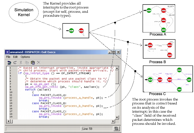
Complex steering of interrupts is best handled by an interrupt-dispatching process as described above. However, KPs provided by the Simulation Kernel’s Interrupt package provide convenient and efficient support that is sufficient for certain simple situations. By using the provided mechanisms, any process may register itself or another process as the direct recipient of appropriate interrupts.
Specifically, two KPs are provided to request that the Kernel automatically invoke a particular process based on the type of interrupt or based on the input on which an interrupt arrives. Steering based on interrupt type is supported by the KP op_intrpt_type_register(), and all interrupt types except for self, process, and procedure are supported. For stream and statistic interrupts, the KP op_intrpt_port_register() provides additional specificity with regard to the input stream or input statistic associated with the interrupt. When both mechanisms are used and are applicable, port registration has precedence over type registration. Automatic interrupt steering is described in detail in Chapter 4 “Modeling Framework” on page 80.
Local Process Resources
Processes always operate within the context of a QP. The QP object provides the processes that it contains with certain resources that are implicitly part of each process’ environment. These resources are described in this section.
Input and Output Streams
Packet streams are objects that exist in the Node Editor and are used to connect modules together. The packet streams support error-free transfer of packets between modules, and can also delay the arrival of the packet at the destination module. Packet streams connect to constructs in the source and destination modules which are called output and input streams respectively.
An input stream of a QP is capable of receiving packets from external sources. The packets are automatically queued within the input stream in first-in-first-out order and are provided to any process within the QP upon request. Input streams accept packets from two sources: packet stream objects and the remote delivery service provided by op_pk_deliver() and related Kernel Procedures. A QP may have any number of input streams that are physically attached to packet stream objects. In addition, input streams are dynamically allocated as necessary to support packet deliveries, because the Simulation Kernel has no prior knowledge of the range of input streams that will be delivered to or accessed.
Figure 95: Queue/Processor Input Streams
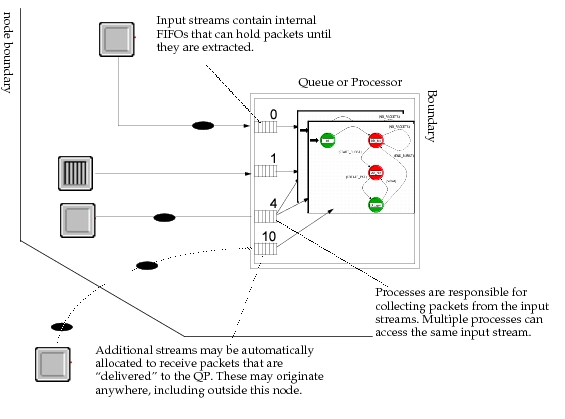
When packets are received on an input stream, one of the processes in the receiving QP is usually invoked with a stream interrupt. The process may determine which input stream received the new packet by calling the KP op_intrpt_strm(). Input streams are referenced using non-negative integer indices. Processes may obtain the earliest arriving packet that remains in an input stream of their QP by calling the Kernel Procedure op_pk_get() and referencing the correct input stream index. The KP op_strm_pksize() can be used to determine the number of packets still remaining in the input stream.
The opposite side of a packet stream attaches to an output stream construct. Output streams support communication of packets via the Kernel Procedures op_pk_send(), op_pk_send_delayed(), op_pk_send_forced(), and op_pk_send_quiet(). Like input streams, output streams are referenced by nonnegative indices; however only output streams that are actually physically connected to outgoing packet stream objects in the node domain are valid.
Output and input streams may also be referenced when the stream accessing mechanism is used. A QP can use stream accessing to signal to another QP that it should forward a packet on one of its output streams. Assuming that module S is the source of a packet stream and D is its destination, the sequence of operations is typically as follows:
- D calls the KP op_strm_access(), to request that S send a packet to it over the stream that connects them. When calling the KP, D specifies the index of the input stream on which it wishes to receive the packet.
- As soon as D calls op_strm_access(), a forced interrupt is generated for S. This means that D’s execution is temporarily suspended to allow S to respond (see the Modeling Framework section for more information on forced interrupts). The type of this interrupt is an access interrupt. S calls op_intrpt_strm() to determine on which output stream the packet is being requested. S then responds to the access interrupt by sending a packet on that output stream, if it so chooses. To send the packet, S must use op_pk_send_quiet() because it has to avoid causing an interrupt for D which is in a suspended state. Note that S could take other actions if desired, as well. S blocks in an unforced state.
- D regains control immediately when S blocks and resumes execution immediately after the point where it called op_strm_access(). D checks its input stream to determine if one or more packets have arrived, typically using the KP op_strm_pksize(). If any packets are present, it may retrieve them from its input stream using the KP op_pk_get().
Input Statistics and Local Output Statistics
Input statistics are constructs that are internal to QPs and that accept numeric values sent by other modules (not necessarily QPs) in the same node. Input statistics are generally used to monitor performance metrics or status signals generated by other modules. The values are conveyed by statistic wire objects that connect the source and destination module. A destination module’s input statistic is capable of retaining only the last value that it receives (i.e., no buffering of values is provided). This latest value is always available to any process in the QP by calling the KP op_stat_local_read().
Each QP has exactly 100 input statistics, each of which can be connected to any number of statistic wires.The input statistics are referenced by integer indices in the range 0 to 99. These indices correspond to the “dest stat” attribute of the statistic wire object in the Node Domain. When multiple statistic wires are connected to one input statistic, the latest value of the most recently updated statistic is the one that is stored in the input statistic at any given time (note that a statistic may be updated without necessarily changing its value).
Changes in the statistics associated with the statistic wires always result in statistic events for the destination module. Each event may then result in the generation of a statistic interrupt for one of the processes in the receiving QP, depending on the interrupt-generation criteria imposed by the statistic wire (see “Node Domain” for more information on the operation of statistic wires). Upon receiving a statistic interrupt, a process may determine which of the QPs input statistics has received a new value by calling the KP op_intrpt_stat().
Local output statistics and input statistics form opposite ends of a statistic wire that connects to QPs. The “Local” qualifier is used to distinguish these output statistics from global statistics that can be shared by multiple QPs across the system model. Local output statistics provide the ability to report user-defined statistics that are private for each QP.
A local statistic can be tapped by statistic probes to contribute to a simulation’s output file, as well as by a statistic animation probe to generate an animated view of the statistic as it changes over the course of the simulation. Local statistics can also be connected via statistic wires to the input statistics of other QP modules in the same node, allowing values to be dynamically communicated to the destination modules as they are updated. Processes can update local output statistics by calling the KPs op_stat_write() or op_stat_write_t(). Each local output statistic can feed multiple statistic wires and probes in any combination. As the statistic’s value is updated, each destination separately receives correct notification.
Each QP can maintain any number of local output statistics. If multiple processes coexist within the QP, the output statistics are shared by all of these processes. In other words, any of the processes may update any of the output statistics, if needed. Processes must declare the local output statistics they intend to use; the Process Editor provides the “edit local statistics” operation for this purpose. This operation is fully documented in the Editors Reference manual. Each local output statistic may be dimensioned or undimensioned. An undimensioned statistic is simply an individual statistic, which is the most common case. A dimensioned statistic is actually an array of statistics, containing any pre-determined number of individual statistics. The individual statistics are distinguished by their index and can be updated and used independently. Dimensioned statistics provides a more convenient way of handling a large number of similar statistics and are typically used in cases where a process manages a scalable number of entities, such as connections or neighbors. Often, in cases where child processes are used, each child process is responsible for updating one of the output statistics in an array of local output statistics.
To gain access to a statistic to update it, a process must first obtain a corresponding statistic handle. The KP op_stat_reg() allows the process to obtain this handle, which it may then retain (usually as a state variable) for subsequent use.
Global Statistics
Local statistics are ideal for reporting activity that is private to a particular QP at a given location in the system model. However, in many cases, modelers are interested in obtaining quantitative information about the system as a whole. For example, in a network model, we may want to measure the average end-to-end delay experienced by all packets transmitted between applications, regardless of the particular source or destination. Another common statistic of interest is network throughput, which is a measure of the total amount of data the network delivers during a chosen time interval. Often, global statistics are simply averages of local output statistics across many components in the system model. It is common to collect both types of statistics in the same simulation.
Global statistics can be used to feed values to two types of statistics collection probes: global statistic probes and statistic animation probes. Global statistic probes transfer statistic values to the simulation’s output files, allowing them to be analyzed in the Results Browser after simulation. Statistic animation probes allow dynamic viewing of the statistic during simulation.
Modeler provides similar, but separate support for local and global statistics. As with local output statistics, each process model is expected to declare the global statistics that it expects to update during simulation. This is done using the Process Editor’s edit global statistics operation which is fully documented in the Editors Reference manual. Global statistics are accessed via a statistic handle which is obtained via the KP op_stat_reg(). To obtain the handle, the name and group of the statistic is specified; if different processes elsewhere in the system model specify the same name and group when calling op_stat_reg(), then they will obtain the same statistic handle, providing a “rendez-vous” mechanism based on the statistic name. The separate processes may then use the handle when calling op_stat_write(); the values provided by all of the processes are merged into one series of values in the simulation’s output file, or in the statistic’s animation. See “Discrete Event Simulation API” for more information about working with global statistics.
Subqueues
Queue modules may be configured within the node domain to contain any number of subqueues that allow packets to be stored in an organized manner. All processes within a queue module have equal access to the subqueues and may insert and extract packets as required to implement a particular queuing policy. The Q and Subq packages of Kernel Procedures support processes that operate on subqueues. See “Discrete Event Simulation API” for detailed information about these Kernel Procedures. Also see the Node Domain Definitions section for a detailed explanation of how queues and subqueues are structured.
Attributes
Like all objects, QPs have a set of attributes that specify some of their fundamental characteristics. All processes within a QP may modify and obtain the values of these attributes by calling the KPs op_ima_obj_attr_set() and op_ima_obj_attr_get(), respectively.
Built-in attributes are predefined and similar for every QP, though their values are assigned independently on a per-QP basis. Model attributes can be declared by the modeler to support modeling of application-specific object characteristics. The Process Editor’s “edit model attributes” operation is provided for this purpose. For more information about this operation, see Editors Reference manual.
Model attributes are inherited by QPs from their assigned process models. This set of attributes is formed from the process model attributes of the root process as well as from those of its child process models. To avoid attribute naming conflicts between the various processes, attribute names are prefixed with the name of the process models that define them (except in the case of the root process).
Model attributes have a scope that is local to each QP. That is, for each QP that uses a process model, private copies of the process model’s attribute are created for the QP and appended to its attribute list. They appear together with the QPs built-in attributes and can be treated in an identical manner. Changes to the attribute in one QP have no effect on the same attributes in any other QP.
Modeler also provides process models with a globally scoped attribute mechanism. These attributes, called simulation attributes, are declared by each process model that requires them. Unlike process model attributes, simulation attributes are read-only. Their purpose is to provide a parameterization mechanism at the system level, rather than at the level of system building blocks. In other words, if the designer of a process model wishes to create a parameter which is to be shared by many entities in the system model, it can declare a corresponding simulation attribute. If multiple process models declare the same simulation attribute (i.e., using identical names), Modeler will detect this and create only one attribute which is implicitly shared by all the process models. Simulation attribute values can be set at simulation run time to complete the specification of the system model. Different values may be specified for each new simulation, providing a mechanism for automatically iterating the system model through a series of experiments.
Declaration of simulation attributes is performed using the “edit simulation attributes” operation, which is described in detail in Editors Reference. When processes want to obtain the value of a simulation attribute, they must call the KP op_ima_sim_attr_get() and refer to the attribute using the correct declared name. If the value of the simulation attribute has not been specified as part of the simulation environment attributes, op_ima_sim_attr_get() will cause the Simulation Kernel to prompt for an assignment from the user. Because simulation attribute values do not change after a simulation starts, processes usually obtain these values once and store them in state variables if they need to use them again at a later time. See “Discrete Event Simulation API” for more information.
Because simulation attributes, and attributes in general, are essentially inputs to the system model and the simulation, they are often of interest to record as part of a simulation’s output file. This allows the simulation inputs and output (i.e., recorded statistics) to be viewed together and dependences between them to be analyzed. Modeler provides a special probe, called an attribute probe, for this purpose. Attribute probes record attribute values as scalar statistics. See “Simulation Design” for more information on attribute probes.
External System Interface Resources
In queues and processors, the process model fills the role of a behavioral model for the QP. For esys modules, however, the process model can also fulfill an additional role. Each esys module has an ESD model attribute that can contain the model name for an external system definition. For an esys module, a process model handles all data going to and coming from the external system. The process model formats data for the external system and is responsible for handling the data that it receives from the external system during a cosimulation.
Because esys modules have all the functionality of queues and processors, you can use esys modules in your node models if there is any chance that you will want to incorporate an external system into the node in the future. An esys module acts just like a queue when its “esd model” attribute has the value NONE. Later, if you want to add an external system, you can use a dynamic process to handle the necessary data exchange with the external simulator. Therefore, an esys module can use processes to both model behavior and interact with external systems.
The rest of this section explains how you can use process models to interact with external systems. Such process models do two functions:
- Read values from and write values to esys interfaces
- Transform values between the format needed at the esys interface level (for example, a bit vector) and the format used by the model (for example, a packet)
While an esys module’s process model is always responsible for placing data on esys interfaces and retrieving values from them, the role that the process model plays in manipulating data can vary. The process model can either place values it receives directly onto esys interfaces just as it receives them, or the process model can transform the data before sending it to the external system. The degree to which the process model is involved with data transformation is up to the modeler.
“External System Package” describes a family of KPs that enables you write values to esys interfaces and retrieve values from them. An esys interface can contain only one value at a time unless it is a vector interface, in which case it can contain multiple values. The KPs op_esys_interface_value_get() and op_esys_interface_value_set() let you read data from and write data to an esys interface. Other KPs enable you to work with groups of data or vector interfaces. More details on working with data and esys interfaces are available in “External System Domain”.
In most cases, the data that esys interfaces exchange is not directly meaningful to Modeler. Because an external system might have little use for a packet, for example, the packet must first be transformed to a format that the other system can understand before being placed on an esys interface. Likewise, data coming from the external system will usually need to be transformed so that it is meaningful to Modeler. An esys module’s process model is responsible for handling these conversions. The KPs op_vvec_from_value() and op_vvec_to_value() make it possible to convert ordinary values to their bit representations and back again. A variety of other value vector KPs enable you to manipulate and transform value vectors, which you can use with external systems or for other purposes. See “Value Vector Package”.
A primary concern when preparing values to place on esys interfaces is the data type of the esys interfaces in question. Because each esys interface can hold values of only one data type, the key issue when preparing data to exchange is how to convert the information that you want to convey from Modeler into information of the correct data type. When receiving data from an external system, all the data coming from the output esys interface will also be of only one type. The process model, then, must convert Modeler data structures (such as ICIs, scalars, and packets) and user data structures to values of one data type before sending them to an esys interface. The process model must also do the reverse, converting values of one data type back to Modeler and user data structures when it receives data from the external system. Strategies for this type of conversion are described in “External System Domain”.
Process Model Components
Process models are specifications for the dynamic behavior of processes. To be complete, a process model must describe the actions that a process will implement under all possible circumstances. In many cases, processes that are executing within discrete event simulations represent a real-world equivalent protocol or algorithm; the formal specification of such a protocol or algorithm is a higher-level specification that stipulates the requirements that must be met by a process implementation to be used in a standardized fashion. To differentiate such a specification from a model specification developed in Modeler, the formal specification will be referred to as a standard. In other words, a standard describes the requirements that apply to real world processes, and therefore also to the models of those processes. Some examples of standards are the IEEE 802 local area network protocol standards, or the RFC documents for the TCP/IP protocol suite. The academic description of an algorithm such as Bellman-Ford Routing would also be considered a standard according to this definition. In fact, any set of requirements that apply to the actions and interactions of a process can be called a standard for the implementations of that process.
Process models are developed to represent real-world existing or planned systems and therefore may at some level be considered to be implementations, or partial implementations, of the same standards as their real-world counterparts. Strictly speaking, processes that are representing existing and known real-world counterparts, are models of those implementations, rather than implementations of the standard. Therefore, a good model of an existing real-world process should replicate any flaws that the real-world process has relative to the standard that it implements. This would allow it to predict behavior that results from the flaw.
In some cases, process models are developed to represent hypothetical processes that could occur in the real world. The modeler may be interested, for example in predicting the performance of a proposed protocol for which no real-world implementations may yet exist. In these cases, process models can themselves be considered to be implementations of the standard from which they are derived. Similarly, a process model may be developed to provide a generic implementation of a standard for use as a basic library component. Such a process would also be considered a direct implementation of a standard, because it is not patterned off of any existing real-world implementations. Most example models provided with Modeler that have to do with standards, such as X.25, Ethernet, ATM, TCP/IP, etc., fall into this category.
Regardless of whether a process model strives to represent a real-world implementation or a standard, the actions that it is required to implement and the timing that underlies these actions may be quite complex and may vary significantly from application to application. Therefore, if one representation convention, or language, is used to define all such process models, it must be extremely versatile. Modeler supports one language for developing models of processes. This language, called Proto-C, is supported by the Process Editor which is integrated into the Modeler application. Proto-C provides a powerful and efficient method for describing the behavior of discrete event systems; it offers the following major features:
- Based on state transition diagrams (STDs) – also referred to as finite state machines (FSMs). This is the prevailing description method for discrete-event systems that maintain state information (i.e., information accumulated over the past). It is used in specifying and developing a wide range of software and hardware systems because of its simplicity, its propensity for intuitive graphical representation, and its ability to effectively break down complexity.
- Combined graphical/textual representation – Proto-C process models depict state-transitions in a graphical format to support visualization of top-level control flow. However, because graphical representations generally do not efficiently or intuitively describe detailed actions or decision-making, Proto-C supports textual specifications of these aspects of a process. Textual specification occurs within the states and on the transitions of the diagram and is based on a powerful library of simulation and distributed-system related procedures, described in “Discrete Event Simulation API”. In addition, the full general computational capability of the C and C++ languages is retained by Proto-C to guarantee sufficient flexibility for all discrete-event applications.
- Ability to represent general state information – the state information of a process is the set of data that has been generated by or provided to the process, and that the process has decided to retain. Traditional state-transition diagrams represent the complete state of a system by identifying which of a limited set of states is occupied at any given time; this is impractical for systems with complex state, and insufficient for systems with dynamically expanding state. Proto-C therefore uses state occupancy representation only to represent high-level modes of a system, and provides a more powerful mechanism to describe general state information. Models may declare any amount of state information as variables whose datatypes are provided by Modeler, the C and C++ languages, or custom definitions. The state variables may be given general names and referenced symbolically throughout the process model. In addition, variables can be assigned to dynamically allocated memory to store state information that grows over time.
- Dynamic process creation – processes may be created dynamically to partition interrupt handling or to provide additional independent contexts as new tasks arise.
- Efficient execution – Proto-C diagrams and the logic contained within are translated to the C and C++ languages with minimal overhead, allowing them to execute extremely efficiently. In particular, state information access, and control-flow statements (e.g.,
ifstatements with conditional clauses, andforloops that sequence through multiple operations) are implemented in a direct manner to avoid any loss of performance.
State Transition Diagrams
Proto-C models consist of two basic component types: states and transitions, hence the name state transition diagram (STD). States are generally used to represent the top-level modes that a process can enter. Transitions specify the changes in state that are possible for the process. STDs are graphically depicted in the Process Editor.
There are other important aspects of Proto-C process models that are not represented graphically. These include actions associated with each state, variable and attribute declarations, and common definitions of expressions and functions. This section provides detailed information on the capabilities and applications of these features.
Forced and Unforced States
In a general sense the word state refers to the information that a process may have accumulated over the time that it has existed. The process’ state may not include all information to which the process has had access, but only that which it has chosen to retain. State information may be continually updated as new events occur and data becomes available. In terms of a state transition diagram (STD), the word state refers to an object that corresponds to one of the primary modes or situations that a process may find itself in. States are mutually exclusive and complementary, meaning that a process is always in exactly one state: more than one state may never be occupied at a time. The process can move between states in response to the interrupts that it receives. The transitions that depart from a state indicate which states may be occupied next, and the condition that each change requires.
Specifications of actions may be associated with each Proto-C state. In Proto-C terminology, actions are called executives. The executives of a state are split into two sections, called enter executives and exit executives. As the names indicate, a state’s enter executives are executed when a process enters the state, and its exit executives are executed when the process leaves to follow one of the outgoing transitions.
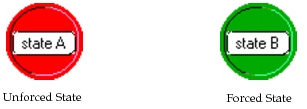
Proto-C defines two types of states, called forced and unforced, that differ in execution-timing. In Proto-C diagrams, forced states are graphically represented as green circles, and unforced states are drawn as red circles. On monochrome displays and hard copy, forced states are dark and unforced states are light.
Figure 96: Graphical Representation of Forced and Unforced States
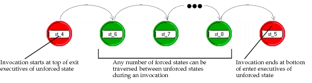
Unforced states allow a pause between the enter executives and exit executives, and thus can model true states of a system. After a process has completed the enter executives of an unforced state, it blocks and returns control to the previous context that invoked it. This context may be another process that invoked this one by calling the KP op_pro_invoke(); or if the process was invoked by the Simulation Kernel, blocking signifies the end of the current event and the Kernel may select a new event to begin its execution. At this point, the process remains suspended until a new invocation causes it to progress into the exit executives of its current state. The following diagram depicts the flow of execution through the unforced states of an STD as interrupts cause the process to advance.
Figure 97: Execution Flow through Unforced States
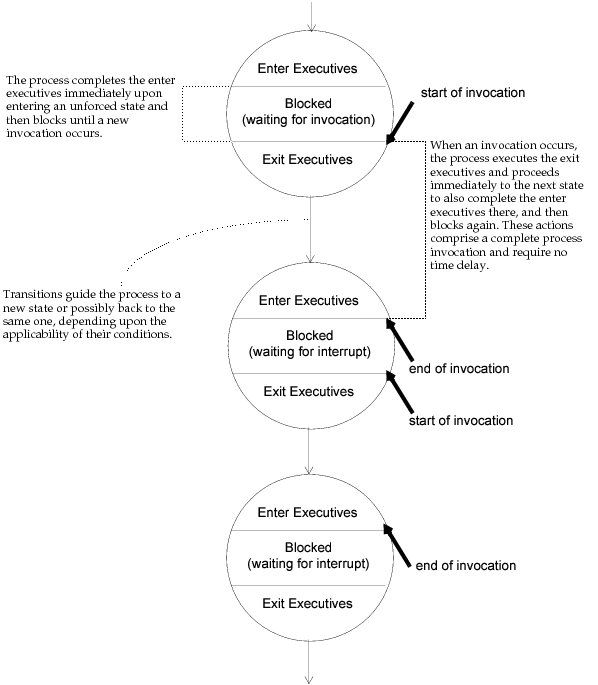
The diagram clearly shows the starting and stopping points of a process’ invocation. In all cases (except the initial invocation), when a process is invoked, it is poised to begin executing the exit executives of its current state. It then progresses until it completes the enter executives of an unforced state where it again blocks. Therefore if only unforced states are involved, the cycle is as follows:
- exit executives of current state
- transition to next state
- enter executives of next state
Forced states are so called because they do not allow the process to wait. They therefore cannot be used to represent modes of the system that persist for any duration. In other words, the exit executives of a forced state are executed by a process immediately upon completion of the enter executives. Therefore the exit executives of a forced state are generally left blank, because they are equivalent to the same statements placed at the end of the enter executives. Because forced states cannot represent actual system states, they are not generally used as much as unforced states. However they are useful in certain cases to graphically separate actions or control flow decisions that are common to several unforced states; graphically separating out definitions of decisions or actions this way can sometimes provide better modularity of specification, as well a more visually informative state transition diagram.
The introduction of forced states causes only a minor adjustment in the execution flow depicted in the above diagram. Unforced states still represent the starting and stopping points of invocations; however any number of forced states may be traversed between them. This is illustrated in the following figure.
Figure 98: Execution Flow through Combination of Unforced and Forced States
Initial State
One special state, called the initial state, must be designated in each process model. An existing state may be assigned this role at any time by using the “set initial state” operation of the Process Editor. Graphically, the initial state is identified by a large arrow located at its immediate left, as shown in Figure 99.
Figure 99: Graphical Representation of Initial State
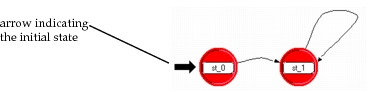
The initial state is the point at which execution begins on the first invocation of the process. It has no special significance for any subsequent invocations, and may otherwise play the role of a normal state. However, because this state usually contains executive statements performing initializations that should occur only once, most models do not include transitions that lead back to it.
Upon receipt of the first interrupt, entry into the initial state takes place at the beginning of the enter executives. Some models devote this state only to initialization actions, and expect that a “begin simulation interrupt” will be provided exclusively for the purpose of completing these actions at time zero. The issue of whether such an interrupt is expected and the related issue of whether the initial state should be forced or unforced must be treated carefully to avoid mishandling the first interrupt. This section uses several different approaches. In describing these approaches, interrupts other than “begin simulation” interrupts are referred to as mainstream interrupts.
-
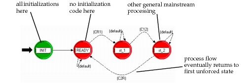
The initial state is forced, and a begin simulation interrupt is expected – Because the initial state is forced, the process necessarily proceeds to a second state as soon as initializations are complete. The enter executives of this second state must not do actions related to the processing of mainstream interrupts because these actions would be (incorrectly) executed at initialization. Typically, the second state is an unforced state that acts as a “ready” position for the process to handle subsequent mainstream interrupts. This approach makes sense for cases where the first unforced state entered after initialization is also reentered for later mainstream processing. Were this not the case, the initial and second state could simply be collapsed into one unforced initial state.
Figure 100: Initialization Strategy 1: Forced Initial State / Begin Sim. Interrupt
-
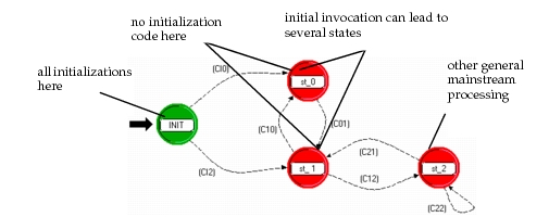
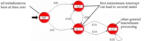
The initial state is forced, and a begin simulation interrupt is not expected – As in the previous case, the process will proceed to a second state immediately after the initial state has completed; however, because the initial interrupt is a mainstream interrupt, it is correct to process this interrupt by performing additional actions. Therefore, the conditional transitions out of the initial state may guide the process into several possible second states, where processing of the interrupt can take place. Note that the limitation presented by this scheme is that initializations are not performed until the first mainstream interrupt occurs, which may be well after time zero.
Figure 101: Initialization Strategy 2: Forced Initial State / No Begin Sim. Interrupt
-
The initial state is unforced, and a begin simulation interrupt is expected – In this configuration, initialization statements placed in the enter executives will complete at time zero, after which the process will block until the arrival of the first mainstream interrupt. Therefore the exit executives of the initial state should be appropriately specified for handling of a mainstream interrupt; they may simply be empty in which case the interrupt handling code must be in the enter executives of the state that follows or in the transition executives. Like the previous approach, this organization makes sense when the first mainstream interrupt may lead the process into several different states; however note that it accomplishes initialization at time zero, rather than waiting for a mainstream interrupt. Note also, that this approach is usually not correct if the initial state is to be reentered during processing of later mainstream interrupts, because the initialization statements in the enter executives would be executed repeatedly.
Figure 102: Initialization Strategy 3: Unforced Initial State / Begin Sim. Interrupt
-
The initial state is unforced, and a begin simulation interrupt is not expected – This is an unusual approach because it requires a mainstream interrupt to do initializations, and yet has the process block without proceeding on to other states. Therefore, any processing associated with the first mainstream interrupt must be embedded in the enter executives of the initial state; if this processing is generic and appears elsewhere in the model (i.e, for steady-state processing of the same sort of interrupt), then it may need to be redundantly specified.
Note that begin simulation interrupts are controlled within the node domain by assigning the correct value to the “begsim intrpt” attribute of processor and queue modules. Also, begin simulation interrupts cannot be enabled for dynamically created processes (i.e., the “begsim intrpt” attribute applies only to the root process of a QP); however, their effect can be emulated for such processes by having the parent process do an invocation via op_pro_invoke() immediately after creation via op_pro_create(). Therefore the above approaches to organizing a process’ initialization stages is applicable to dynamic processes as well.
Improper configuration of the initialization stages can result in serious logical errors for a process. In particular, if a process that expects a begin simulation interrupt (or equivalent invocation) does not receive it (e.g., because the “begsim intrpt” attribute is not enabled), it may misinterpret the first mainstream interrupt as the interrupt it expected. Typically in such cases, initialization is still performed correctly because the process simply assumes it has received the expected indication to do initializations. However, the mainstream interrupt is likely to be ignored by the process, which can lead to loss of critical information and/or omission of critical early actions that should have been taken by the process.
One particular example of this problem occurs when the first mainstream interrupt that occurs is a stream interrupt, indicating the arrival of a packet at one of the QPs input streams. If the process assumes a begin simulation interrupt has occurred instead, the arriving packet is likely to be ignored and will remain in the input stream. Subsequent stream interrupts that are correctly interpreted will cause the process to try to acquire the arriving packets from the input stream; however, because streams queue packets in a first-in-first-out order, the ignored packet will be obtained instead. Therefore, models that exhibit this error can be identified by a “shift” in the packet processing. Paradoxically, one of the effects of this shift is that processes that receive packets infrequently tend to forward them with greater delay, because each packet must wait for the following one to trigger its processing; this behavior is counterintuitive for some simulation studies that measure cumulative delay of packets through a system, because in general less frequent arrivals correspond to a lightly loaded system, which in turn implies lower delay through the system.
Transitions
Transitions describe the possible movement of a process from state to state and the conditions under which such changes may take place. There are four components to a transition’s specification: a source state, a destination state, a condition expression, and an executive expression. The specification may be read as follows: when in the source state, if the condition is true, implement the executive expression and transfer control to the destination state.
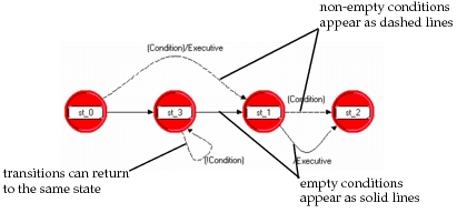
In the Process Editor, transitions are specified graphically. Each state may have any number of outgoing and incoming transitions depicted as directed arcs with the arrow pointing toward the destination state. The condition and executive expressions appear in a combined label next to the arc. The tool always places the condition expression within parentheses and precedes the executive expression by a forward slash (‘/’) to separate the two components. Transitions that have non-empty condition expressions are depicted as dashed arcs; those without conditions are depicted as solid arcs, as shown in the following diagram.
Figure 103: Representation of Transitions
A transition’s condition is evaluated as a boolean expression to decide whether the process should enter the transition’s destination state. A process evaluates outgoing transitions after the exit executive statements of the source state have completed. For forced states, enter and exit executives are executed in immediate succession, and so both executive blocks and the transition evaluation can be viewed as one logical series of actions (although exit executives are usually empty for forced states). For unforced states, a pause occurs between the enter and exit executives, and so only the latter can be grouped with the transitions.
Transition condition expressions may be complex combinations of criteria that involve state variables of the process, attributes of the current interrupt, and other information stored in shared or global memory. It is also possible for conditions to be based on computations of any complexity by calling a user-defined procedure that returns a boolean value (typically, such a procedure would be placed in the function block of the process model). Alternatively, computations that support condition expressions may be placed at the end of the exit executives of a transition’s source state, because these are executed immediately before the conditions are evaluated.
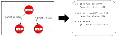
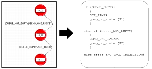
All transitions that depart from a state are evaluated before a process may progress to any transition destination. This allows the detection of two types of errors and assures that behavior is independent of the order in which the transition conditions are evaluated. If none of the conditions have a TRUE value (a nonzero value as a C or C++ language expression), then an error message to this effect will be generated by the process, because it is impossible for it to continue execution. Similarly, if more than one transition condition has a TRUE value, an error message will be issued. Both of these errors are considered sufficiently serious to cause the simulation to halt. It is therefore important that the transitions that emanate from a state should collectively be mutually exclusive at the time they are evaluated (no two can simultaneously be true), and complementary (at least one is necessarily true). The following equivalence between an STD fragment and a pseudo-code fragment shows the logic that is applied to evaluate multiple outgoing transitions.
Figure 104: Pseudo-Code Equivalent of Multiple Transition Configuration
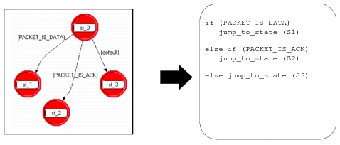
A special condition called default is provided to represent the complement of the conditions associated with the defined transitions leaving a state. Each state should have at most one outgoing default transition. This is a useful mechanism to represent complementary conditions when they are complex, and ensures that the process will not encounter an error at the state of interest due to a missing TRUE transition. Default transitions succeed only if all other transitions conditions are false, as shown by the pseudo-code example below:
Figure 105: Pseudo-Code Equivalent of Multiple Transition Configuration with Default
As a final note on condition expressions, transitions that are configured with an empty condition attribute are equivalent to transitions whose conditions always evaluate true. These are referred to as unconditional transitions. It follows from the previous material that if a state has an unconditional transition departing from it, that it may support no other outgoing transitions.
Each transition incorporates an attribute that supports the specification of an executive statement. A transition’s executive is carried out at the time that a process decides to traverse the transition. In other words, after all outgoing transitions have been evaluated, the process selects one of them, implements its executive statement if there is one, and advances to the enter executives of its destination state. This sequence is described below in the form of pseudo-code for a simple pair of transitions.
Transition executives are useful to associate an action with a state, but only when it is entered or exited for a particular reason. Actually incorporating the action into the state’s enter or exit executives instead would cause it to be executed regardless of the reason for which the state was entered/exited, which may be undesirable in some cases.
Figure 106: Pseudo-Code Equivalent of Transitions with Executives
Using Macros to Define Complex or Recurring Expressions
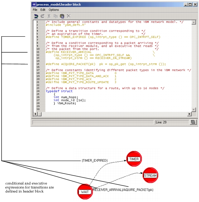
In the examples above, condition and executive expressions consist only of “English-like” text, and at first sight do not appear as C language programmatic expressions. The technique used in these examples, and typically used in most process models, is to define macros whose names represent underlying expressions. Proto-C simply “passes through” the macro definition capability of the C language to support this practice.
Almost all macros used by a Proto-C model are defined in its header block. The header block is a free-form area for C or C++ language code, similar to the top portion of a C or C++ file. Macros are generally used to represent constants, transition conditions, transition executives, or commonly performed operations.
Macros defined directly within the header block begin with the #define C and C++ preprocessor directive. Macros may also be defined in external definitions files (files with a “.h” suffix in C and C++) and included through the header block by using the #include preprocessor directive. The external file inclusion method is useful when multiple process models must share a consistent set of definitions; this avoids having to enter and maintain identical definitions in each process’ header block. The following header block fragment provides an example of typical Proto-C macro definitions.
Figure 107: Macro Definitions within Process Model Header Block
Variables
Proto-C processes have access to several forms of memory to store information. Each form of memory has different properties that make it correct for particular uses. Some of these memory forms allow information to be declared and manipulated directly as ordinary names; these forms of storage are referred to as variables. Proto-C processes can make use of three distinct categories of variables called state variables, temporary variables, and global variables. The following table shows these types of variables and the sections of code where they can be accessed.
Table 44: Visibility of State, Temporary and Global Variables
| Type of Variable | Visibility | ||
|---|---|---|---|
| State executives | Functions in function block | Functions in external files (.ex.c files) | |
| temporary | X | ||
| state | X | X | |
| global (as defined in external header files or in the Header Block) | X | X | X (as long as “extern” is used) |
Variable Components
All variables, regardless of their category, have a name, a datatype, and a value. The name and datatype of a variable remain fixed throughout the life of a process; the value component is the only one that may change.
- Name – unlike attributes, variables can be accessed without the use of any Kernel Procedures. Instead, an ordinary reference to a variable’s name implicitly signifies a reference to its value. Variable names are defined as part of a mechanism called declaration; each of the three variable categories uses a slightly different declaration mechanism to indicate to the process compiler what category applies. The names that are selected can be general alphanumeric character sequences respecting the following rules:
Table 45: Rules for Variable Naming
-
Names must consist of alphanumeric characters only; the underscore character (‘ _ ’) is also allowed. Both upper and lower case are acceptable and are considered distinct.
-
Names must begin with letter characters (i.e., not numbers or ‘ _ ’).
-
Each name must be used in only one declaration (i.e., the same variable name should not be used for more than one of the variable categories in a given process).
-
Datatype – the datatype of a variable specifies the kind of information that it is capable of storing. Modeler provides a number of special datatypes that are predefined for common modeling purposes. Some of the essential datatypes are listed in the following table. See “Discrete Event Simulation API” for a complete listing of predefined datatypes and their usage.
Table 46: Essential Predefined Datatypes for Variables
| Datatype | Description |
|---|---|
| Distribution | Loaded Probability Density Function. |
| Evhandle | Handle providing access to a scheduled event (e.g., supports cancellation). |
| Ici | Group of attributes used to associate additional user-defined information with an event. |
| Objid | Unique identifier of a simulation object; used in most operations on objects. |
| Packet | Structured group of data fields representing a message that can flow over packet streams (node domain) and over links (network domain). |
| Compcode | Status value returned by many kernel procedures to indicate success or failure. |
| List | Linked list construct provided by the Prg package of KPs. Useful for managing lists of general user-defined data structures. |
| Stathandle | Handle provided when a local or global statistic is registered. Used to write updated values to the statistic. |
In addition, Proto-C provides completely general data storage by supporting datatypes from the C and C++ languages. This includes not only built-in C and C++ datatypes such as int, double, and char, but also arrays and complex data structures formed from any combination of other datatypes.
Custom data types are usually specified in the header block of a process or in an external definitions file that is included via a #include statement in the header block. In general the C typedef and struct mechanisms are used as shown in the examples below. Consult a C or C++ language reference for complete information on the use of these constructs.
Figure 108: Definition of Custom Datatypes in Header Block
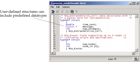
Variables are declared in slightly different formats depending upon their category; declaration mechanisms are explained in each category topic. However, in all cases, declaration requires that the data type and name of a variable be specified. Additionally, a variable may be modified so that it is actually an array of one or more dimensions of its particular data type. In general, the declaration format is as follows:
Figure 109: Declaration Format for Variables
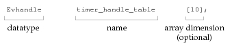
- Value – this term refers to the actual contents of the memory that is associated with a variable. For simple variables this may be an individual number or string of characters; for compound data structures many such items could be involved. The specific nature and organization of a variable’s contents are specified by its datatype. These contents may change over time to store new or updated information, as requires by the process model, hence the name variable.
Operations on Variables
Proto-C variable values are manipulated within the condition and executive statements of states and transitions. The basic operations that can be performed on a variable, regardless of its type, are to obtain its value or to modify its value. Note that the datatype and name of a variable are immutable.
Depending on how a variable name is used in a statement, its value can either be obtained or modified. In general, all variable manipulations follow the conventions of the C language; most C textbooks should therefore provide in-depth coverage of this topic. Briefly, there are two basic forms that support modification of a variable value. The first, and most common is an assignment using the equals (=) operator, several examples of which are shown below:
Figure 110: Assignment of Variable Values with the ‘=’ Operator
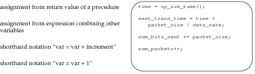
A second method of assignment is designed to allow a procedure to modify a variable’s value rather than modifying it in the local context. This is accomplished by informing the procedure of the memory location at which the variable’s value is stored. Therefore, the procedure can modify the contents of the memory locations and upon returning, the assignment has already been performed. A number of Kernel Procedures use such an interface to support modification of multiple variables in one call (C and C++ functions cannot otherwise return multiple values), or to compute results of several different data types. In the C and C++ languages, the memory location of a variable’s value is obtained by applying the & operator to the variable’s name, as shown in the following examples.
Figure 111: Assignment of Variable Values by Passing Addresses to Procedures
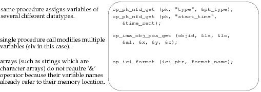
Obtaining the value of a variable is very simple, because a variable’s name actually is a symbol representing its value. In other words, by simply mentioning a variable, the C/C++ language automatically substitutes its current value in the surrounding expression. Note however, that this is true also for modification of a variable using the = operator, as shown above. What differentiates an assignment from an obtainment has therefore more to do with the placement of the variable names relative to the operators in an expression. When the = operator is used, the variable value on the left side of the operator is modified, whereas variable values on the right side are simply obtained (that is, their current values are substituted in the locations where their names appear).
Other commonly performed operations on Proto-C variables include comparison operators such as == (is equal to), != (not equal to), > (greater than), < (less than), >= (greater than or equal to), <= (less than or equal to). Note the difference between the equality test operator which has two side-by-side ‘ = ’ characters and the assignment operator represented by just one such character. The confusion between the two is a source of common errors in process behavior.
In addition, arithmetic operations such as +, -, *, and / are supported, as are all other C/C++ language features. See a C or C++ language reference for an in-depth treatment of these and other operators.
State Variables
Variables that are used to represent the information accumulated and retained by a process are referred to as state variables. This name is due to the fact that these variables, together with the current position of a process within its state transition diagram, represent the complete state of a process at any time. Note that processes might generate or have access to much information over time that does not become encoded into their state; therefore state refers only to the information that the process itself decides to retain by recording it into state variables.
State variables are declared in a dedicated area of a Proto-C model, referred to as the state variable block. New state variables can be declared, or old ones modified by choosing State Variables from the Code Blocks menu of the Process Editor. For details on using this operation, see “State Variables”.
State variables are persistent, meaning that from the perspective of each process, they retain their value over time. They can only be modified by explicit assignment statements that are executed by the process itself. This implies that the values of the state variables of a process are “frozen” when it blocks (i.e., halts execution after completing the enter executives of an unforced state), and found unchanged by the process when it resumes execution at its next invocation (note that, although it is rarely used, the KP op_ima_obj_svar_get() allows this traditional property of state variables to be altered).
An important property of state variables that is necessary for persistence is that they are maintained in a manner that is private for each process. This means that instances of the same process model, even if they exist within the same queue or processor, can store information independently in their variables without conflict, even while referring to them with the same names. In other words, changes made to state variables in one process do not affect the values of variables held by another.
State variables have no particular initial values when a process is invoked for the first time. Because these variables are part of the state of a process, it is the responsibility of the process itself to assign consistent initial values to them during the first invocation. In fact, this is usually one of the principal activities conducted in the executive statements of the initial state. Note that in contrast to temporary and global variables, it is not possible to incorporate an automatic initialization of state variables into their declaration.
An important caution applies when selecting names for state variables due to the underlying method by which they are implemented. It is important to avoid naming conflicts with symbols used elsewhere in the process model. In particular, a state variable name
- must not be identical to the names of temporary variables, functions, function arguments, structure fields, or local variables of functions that appear elsewhere in the model
- must not appear as a substring in function block code
Either of these conditions will cause compilation errors.
Temporary Variables
A process may declare temporary variables to store information that does not require persistence. Temporary variables are not guaranteed to have any particular set of values when a process model is invoked. In particular, the values that were assigned to these variables by the same process during its previous invocation may have been changed.
Because they are not persistent, temporary variables are useful only as “scratch” storage to facilitate computation of complex expressions or to hold information within the time frame of one process invocation. For example, an integer variable used as the index of a loop would generally be a temporary variable; a packet that is obtained, examined, modified, and sent again all in one invocation, would also be a temporary variable. To decide if a process model should declare a variable under the state or temporary category, the developer should determine if there are cases in which the variable needs to retain its value from one invocation to the next. If this is the case, then a state variable must be used; otherwise a temporary variable may be used. If there is doubt concerning a variable’s declaration, state variables may always safely be used; note however that a state variable requires a memory allocation of corresponding size that will last as long as the process exists, whereas a temporary variable requires no additional memory.
Temporary variables are declared in an editor pad that appears as a result of using the “edit temporary variables” operation. An example of temporary variable declarations appears below. Declaration of any predefined C/C++ and Riverbed datatypes as well as user-defined datatypes is possible. Note that the backslash character (‘\’) does not precede the variable name as it does in the case of state variables.
Automatic initialization of temporary variables is possible by incorporating an assignment into the declaration, as shown in the example below. This initialization takes place each time that a process is invoked.
Figure 112: Temporary Variable Declarations
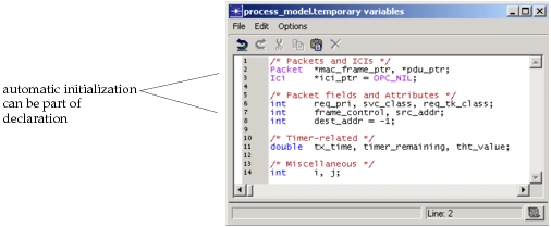
Global Variables
Global variables provide a means for multiple processes in different modules, including processes of different types, to store information in a common location. This is a feature provided directly by the C and C++ languages, which also refers to these types of variables as globals.
Global variables can use any C or Riverbed predefined data type, as well as custom datatypes. Declarations should be entered into a process model’s header block via the “edit header block” operation of the Process Editor. Each global variable should have one principal declaration within the header block of the process model with which it is most closely associated. If other process models also share access to the variable, their header blocks must include an external declaration. There can be any number of process models with external declarations to a global variable, but only one should include a principal declaration. External declarations are identified by the keyword extern, as shown in Figure 113.
As with temporary variables, global variable initializations can be performed by making assignments within the declaration statements. This is possible only within the principal declaration. Initialization takes place before the simulation begins. Additional initializations of globals that are a function of simulation input or model configuration are generally performed by designated processes during their initial invocations.
Figure 113: Declaration of Global Variables in Two Process Header Blocks
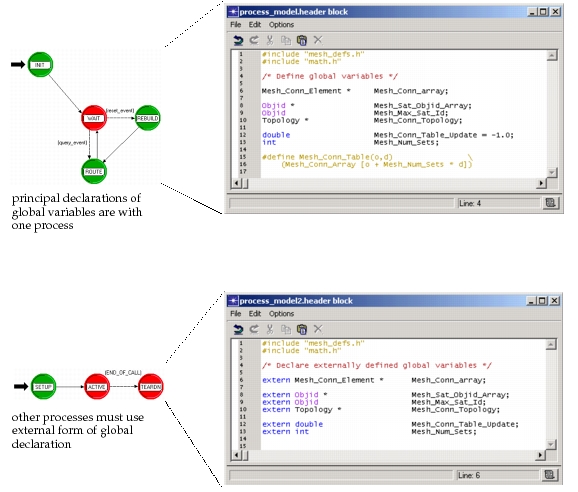
Global variables should be used with care because they can create dependencies among processes. In other words, when a process modifies a global variable, the change may have an impact on the operation of other processes. In addition, global variables that are shared across physical boundaries (e.g, across an entire network model) do not always correspond to realistic representations of actual systems. The same data that can be represented by globals in a model might be implemented as distributed storage in an actual system; or if centralized storage is used, delays would be incurred when accessing the data. The model developer must make a judgement regarding the appropriateness of the global variable approach and possibly make corrections for unrealistic effects it introduces.
Global variables also present problems for parallel simulations. See “Global Variables” for details.
Process Model Attributes
Process model designers frequently specify characteristics of a process that require the flexibility to adapt to a variety of situations. For example, communication protocols may provide various options to their users, such as time-out durations, maximum number of retransmissions, window sizes, etc. Similarly, a computer operating system model may offer multiple alternatives for virtual memory size, maximum number of concurrent tasks, etc. Rather than design similar process models that differ in just these features, it is preferable to design parameterized process models. Those characteristics of the process that require variability can be viewed as parameters of the model.
As described in “Modeling Framework”, Modeler provides model attributes for the purpose of developing parameterized models. Process models are the models that typically make most use of this capability, because ultimately, it is user-defined code that must in some way interpret the values of customized attributes to implement variable behavior (in contrast, the variable behavior of standard objects is configured via built-in attributes). It is normally best to define the model attributes in the same model as the code that uses them.
Model attributes can be declared for a process model by using the “edit model attributes” operation of the Process Editor. Each model attribute is defined by specifying a unique name, and properties. The properties allow control over the attribute’s default value, symbol map, numerical range if appropriate, and several other characteristics. See “Modeling Framework” for more information about model attributes and attribute properties.
Figure 114: Process Model Attribute Declaration
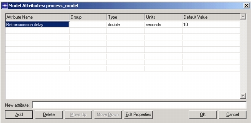
During simulation, process model attributes appear simply as attributes of queues and processor modules. They may be accessed both to modify and to obtain their value by using the KPs op_ima_obj_attr_set() and op_ima_obj_attr_get(), respectively. However, in most cases, process model attributes are never changed during the simulation but instead serve only as parameters that the process uses to configure itself when the simulation begins. Typically, each process that uses model attributes performs these configurations in its initial state, where it loads the values of attributes into a corresponding set of state variables. The state variables are used thereafter because they are more convenient and efficient to access than attributes. A typical example of model attribute loading appears below.
Figure 115: Loading of Process Model Attributes into State Variables at Initialization
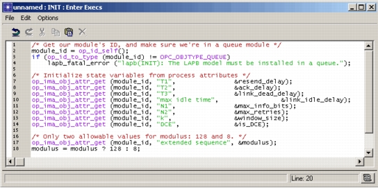
Attribute Interfaces
Each process maintains a set of attribute interfaces that is distinct from its model attributes. As described in “Model Attribute Interfaces”, the attribute interfaces contain attributes promoted from objects within the model, as well as specifications for attributes of the object that will use the model. In the case of a process model, none of the objects within the model (e.g., states and transitions) can promote attributes, and the object that will use the model is a queue or processor. Therefore, the attribute interfaces consist simply of queue and processor attributes. By using the attribute interfaces, the process model developer can specify in advance the values and properties of a queue or processor that will use this model.
Figure 116: Specification of Process Model Attribute Interfaces
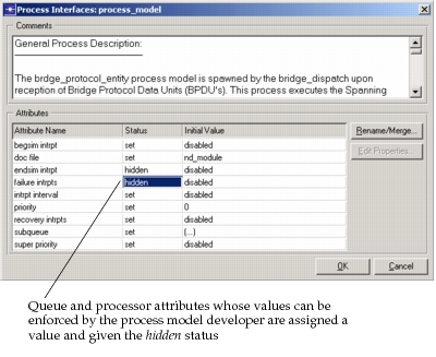
Process model attribute interfaces are frequently used to ensure that queues and processors are properly configured to act as hosts to a given process model. In general attributes that are not relevant to the process model are placed in the “hidden” status to simplify the QPs menu. In many cases, this includes attributes such as “intrpt interval”, “failure intrpts”, “recovery intrpts”, “super priority”. The process model designer generally knows whether the process requires a begin simulation interrupt and whether it supports and end simulation interrupt; the “begsim intrpt” and “endsim intrpt” attributes can be set accordingly and hidden.
Process model attribute interfaces also provide the capability to associate comments with the process model to provide guidance and background information to users of the process model. See “Modeling Framework” for more information about model attribute interfaces.
Modularizing Computations
Certain process models make recurring use of an identical computation in support of a decision or action. Identical does not necessarily mean that the result is always the same, simply that the form of the computation (i.e., the steps into which it can be decomposed) is invariant. However, the data that the computation manipulates may change each time that it is executed. This data is called the input of the computation and each individual data item that comprises the input is referred to as a parameter of the computation.
The most straightforward approach to realizing a process model that has recurring use of the same computation is to simply repeat the specification of the computation in detail at each location where it occurs (i.e., in various executive blocks and on each transition that executes it). However, this approach presents several significant disadvantages:
- It requires redundant entry, lengthening the time required to complete a model’s specification.
- It requires redundant maintenance, meaning that if the computation needs to be changed, to enhance or update the functionality of the model for example, then identical changes must be made in multiple parts of the process model.
- For complex computations, the size of the model may increase appreciably, in turn affecting the total memory requirements of a simulation.
- Process model logic is not streamlined, requiring someone studying the process model (e.g., to understand or upgrade its functionality) to examine or verify significantly more statements.
There are two principal techniques used in Proto-C to streamline recurring specification of identical computations. In both cases, the objective is to encapsulate the specification of the computation into a form that can be reused whenever the result of the computation is needed. Proto-C dynamic processes and C/C++ functions both support this modular computation approach because they can contain general calculations that operate on variable inputs called arguments. Arguments are the parameters of a computation.
Modularizing Computations with Dynamic Processes
Dynamic processes are described in depth in previous parts of this section, as well as in “Modeling Framework”. A brief description of their use for modularizing a computation is presented here.
- A dynamic process that contains all the logic of the computation of interest must be specified. This process should make use of argument memory obtained via the KP op_pro_argmem_access(), to represent the computation’s parameters. In addition, this process should be stateless; this means that it should define no state variables and include only one unforced state to assure that only the arguments of invocation affect each outcome. In other words, there should be no internally accumulated information that can create dependencies between separate invocations.
- A process that requires recurring computations creates a dynamic process of the appropriate type, by calling the KP op_pro_create() and retains the process handle that is returned. This must be done at some time prior to the computation’s first use—usually in the parent process’ initial state.
- Each time that the parent process requires the computation to be performed, it must set up appropriate argument memory and invoke the child process using the KP op_pro_invoke() and the earlier obtained process handle. If required, the child process may return results by modifying the argument memory.
Modularizing recurring computations is not the main application of dynamic processes. Processes are primarily designed for modeling ongoing threads of execution. These threads normally have state memory and therefore do not behave identically on each invocation. However, the dynamic process approach outlined above is followed in some cases as an alternative to using C or C++ functions (described later in this section), because it allows graphical decomposition of a computation's flow of control. Forced states represent simple actions, and decisions about which actions should be performed are encoded in the transitions between states. The following figure show how representing a computation this way resembles the flowcharting approach used as a first step in some computer-program design methods.
Figure 117: Control Flow of Dynamic Process Implementing Modular Computation
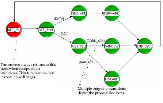
Modularizing Computations with Function Calls
The most common and straightforward approach to modularizing recurring computations is to make use of the function call mechanism provided by the C and C++ languages. Functions (also referred to as procedures) are specifications of computations that may accept parameters, referred to as arguments. Arguments may be of any datatype provided by C, C++, Modeler, or the user’s custom definitions. Depending on the service that is required of them, functions may provide return values that result from their computations or simply do a series of actions and return no result. See a C or C++ reference text for more information about defining functions.
In Proto-C, any number of functions may be specified within a section called the function block of a process model. The function block’s contents can be edited by using the “edit function block” operation of the Process Editor. All normal syntactic rules of the C/C++ programming language apply within this section of the model. However, note that the text that is entered in the function block will appear after that of the header block, allowing the use of data types and macros that are defined therein.
Each function represents a “package” of capability that the logic embedded within the state transition diagram (STD) may call upon. This simplifies the appearance of the STD and allows it to exercise the same functionality in multiple circumstances with minimal additional specifications. For example, an STD may require the same exact series of actions to be applied to a packet while in different states and upon traversing several transitions; by implementing these actions within a function in the function block, the required logic can be developed only once and invoked from each part of the model that requires its execution.
Functions specified within the function block are generally for the use of the process model that they are associated with. However, a function defined in the function block of one process may be called from the STD or even from the function block of another. However, this practice creates dependencies between process models such that the process that actually contains the function’s definition must always be present within a model that also includes the process that calls upon the function. If this rule is not followed, an error relating to the missing function will result when attempting to generate simulations.
A simple solution to the dependencies created by cross-calling of functions is to ensure that each process model is self-sufficient by incorporating all function calls that it requires within its own function block. However, two important caveats apply to this technique: first, if a function appears in the function blocks of multiple process models, then it must have a different name in each one, or the function will be considered to be “multiply defined”, and a corresponding error will occur when attempting to create a simulation executable that includes the conflicting processes. One possible approach to avoiding this problem is to always prefix the names of functions defined within the function block with the name of the process itself. For example, a function that schedules a timeout event for a process called X25 could be called x25_schedule_timeout. Second, redundantly specifying capability by replicating a function in the function blocks of several process models defeats one of the important purposes that suggests the use of functions in the first place; namely, the redundant maintenance and synchronization of the multiple instances can complicate development and maintenance efforts and lead to inconsistencies among the versions.
External Object Files
As an alternative to this approach, the model developer may want to consider defining functions in external object files that are linked into the simulation executable. This allows each function to be developed and maintained in a centralized fashion and still be shared by all process models that require it. It does, however, create a dependency between the process models and the external files that contain the functions. This prevents the process model from being “stand-alone”, which can cause minor complications when sharing the model with other users, for example.
Modeler allows the user to specify those external object files that a model requires at two separate modeling levels. The list of external object files may be specified as part of a network model if desired. However, this approach requires that the user have knowledge of the external files that are implicitly relied upon by the node models that are present. This is not always possible or desirable, particularly when the network level user is not the same individual who developed the embedded process models. This can be a problem for users of other Riverbed analysis software products, who manipulate node and link models but do not normally have knowledge about the make-up of the models. To circumvent this problem, and also to provide a more solid association between the external files and the code that relies upon them, Modeler allows each process model to formally declare the external object files on which it depends. This can be done using the “declare external object files” operation of the “Process Editor”. Declaring external object files allows Modeler to construct the list of external files that are required to construct a complete simulation automatically; this provides transparency to network-level users. See “Simulation Design” for more information about external object files.
Declaring Functions
If functions return values that are not integers (i.e., are of datatypes other than int), these functions should be declared prior to their use. If they are used within the STDs executive and condition statements, corresponding function declarations should be placed in the header block, to ensure that they appear in the correct order. The purpose of a function declaration is to inform the compiler what type of value will be returned. Declaration syntax is shown in the following figure.
Figure 118: Header-Block Declaration of Functions
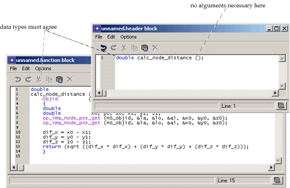
Functions defined within the function block have access to variables on a slightly different basis than the process model with which they are associated. Global variables are available in an identical manner with declarations (either principal or external) required in the header block. Temporary variables of the process are not usable within the function block’s functions. However, each function may of course declare its own local variables. State variables are available to a function block function, but use of direct references to these variables will preclude calls to the function from other processes. In other words, state variables may be accessed only if they belong to the associated process model (i.e., the one in which the function block is included) and in addition, that process model is the one currently executing. Misuse of state variables in the function block can lead to complex simulation errors and should therefore be considered very carefully. A simple way to avoid this issue is to pass the values of state variables to a function as arguments, rather than allowing it to access them directly; similarly, if a calling function would modify state variable values, then the state variables may be passed by address as arguments to the function, or assignments may be performed by higher level code, after the function has returned.
Diagnostic Capabilities
Discrete event simulations automatically incorporate a sophisticated “debugger” called ODB that allows the user to interactively monitor the progress of a simulation and the state of its objects. ODB’s capabilities are exercised from a command line. Most of these capabilities are entirely provided by the Simulation Kernel and require no customization on the part of the developer. However, because processes are user-defined and can store information in proprietary data structures, and because the Simulation Kernel is not capable of knowing which particular information within a process is interesting to report, ODB provides two special commands that can be applied to processes. These commands, called prodiag and proldiag, allow useful reports to be printed about the current state of a user-defined process.
The prodiag and proldiag commands require an argument, which is the process ID of the process of interest. Process IDs can easily be obtained via the promap command of ODB. prodiag and proldiag then execute a series of user-provided statements that have been specified in a special section of the process model, called the diagnostic block. The diagnostic block of a process can be modified by using the “edit diagnostic block” operation of the Process Editor.
Before executing the statements of a process’ diagnostic block, ODB temporarily makes the process active, as if it has been invoked, so that Kernel Procedures such as op_id_self() and op_pro_self() can be used. In addition, state variables of the process may be accessed normally.
General Proto-C logic may be defined in the diagnostic block, although in general, the statements of the diagnostic block are quite simple, because their purpose is simply to report the information that constitutes the state of the process. In some cases, for or while loops are required to report the contents of lists; if statements are also sometimes used to report only information relevant to a given situation. An example of a process model’s diagnostic block is shown in the following figure.
Figure 119: Typical Process Model Diagnostic Block
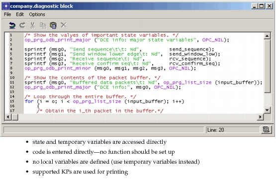
Note from the example that the KPs op_prg_odb_print_major() and op_prg_odb_print_minor() are used to print information rather than the C library function printf(). These two KPs standardize the format of the information that is printed to better integrate it with other output issued by ODB. The example also shows that the diagnostic block is not itself a function and therefore cannot declare local variables. However, it may make use of variables declared in the process model’s temporary variable section.
A more sophisticated version of the prodiag command, called proldiag, is also provided by ODB. proldiag differs from prodiag in that it temporarily activates a debugger label, which can be used to selectively do operations in the diagnostic block. For more information on this topic, see “Simulation Debugger (ODB)” on page 39 and the description of the KP op_prg_odb_ltrace_active() on page 85.