LAN and Cloud Models
Modeler lets you model the end systems of your network in explicit detail, representing each device, if necessary. However, in many simulation studies, you will prefer to abstract local area network infrastructure into one object, called a LAN object. The LAN object models many users on the same LAN, and allows for a server within the LAN as well. However, it does so within one object, dramatically reducing the amount of configuration you need to do to represent your internetwork of LANs. Because fewer objects are present in your network, LAN objects also help reduce the amount of memory needed to do simulation. The following figure shows the types of LAN objects provided for local area network technologies.
Figure 21: LAN Objects Abstract Local Area Infrastructure

Using LAN objects you can quickly generate large amounts of users for your network. Specifically, each LAN object allows you to specify the number of users present within it. You can then assign application traffic to a subset, or all of the users of the LAN. Therefore, scaling the traffic generated by a LAN (to model more users, for example), is a simple matter of increasing the specified number of users. LANs can then be interconnected via switches and routers to carry traffic to and from devices and LANs in other parts of the network.
In a manner similar to the use of LANs, it is sometimes useful to abstract parts of the wide area network infrastructure. Cloud models are special objects in the model library used to represent such infrastructure. They provide high-level characteristics used to simulate the behavior of that portion of the network. The ATM, Frame Relay, and IP model suites all include cloud models.
Figure 22: Cloud Objects Abstract WAN Infrastructure
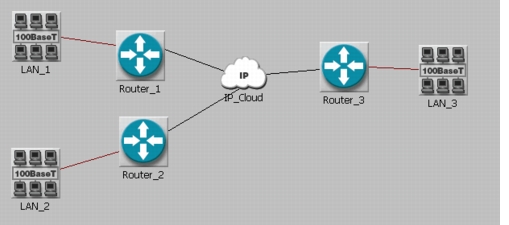
Cloud models can have numerous applications. For example, your backbone network may depend on services delivered by an Internet Service Provider (ISP), which in turn may be connected to a carrier network. Because you do not know the details of the backbone, a cloud node gives you a simpler model without losing any detail.
You may also find cloud models useful if you are more interested in modeling LAN infrastructures than network infrastructures. If your primary focus is on modeling details on LAN traffic flows, you may not want to model the backbone network in minute detail. Representing the backbone with a cloud should suffice.
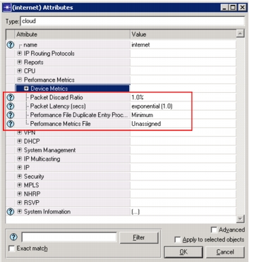
You can simulate a backbone network using two cloud-model attributes, described below. You can specify these through Edit Attributes, which then applies the settings to all packets, or you can specify these through an external file, which then applies to source-destination or ingress-egress pairs.
Figure 23: Cloud Attributes
-
Packet (or Cell) Latency – specifies the one-way delay that each packet experiences while traversing the network. You can run a simple test on your network to determine this setting. First, configure your ping traffic (using an option like IP’s record route) to report the number of hops that a packet traverses. Then measure the response time and number of hops for a typical ping packet sent across the network. (Keep in mind that this response time includes transmission delays at each hop.) After you have these two values, you can use the following equation to compute the actual network latency:
Latency = (Ping Response Time – (Hop Count * (Ping Packet Size/Data Rate)))/2Note: One-way delay is not accurately derived by dividing the RTT by 2, since links are not typically symmetric (i.e., forward and return path are not guaranteed to be the same).
Use the resulting value for the latency parameter. You can also specify any built-in or custom distribution to model variability in the delay.
-
Packet (or Cell) Discard Ratio – specifies the ratio of packets dropped to packets submitted to the network backbone. You can set this value based on your network service provider’s statistics or its traffic-contract guarantees.
You can also import operational delay information and packet loss metrics for cloud models using one of the methods listed below. Either method allows you to specify pair-wise operational delay and packet loss metrics for cloud models and to apply these metrics on each packet that traverses the cloud during a simulation. The packet-loss and latency characteristics of cloud models can be modeled either as single settings that are applied to all routed packets or as separate settings for individual source and destination pairs using a .gdf file
- Explicitly Specify Performance Metrics on a Cloud
- Generate Performance Metrics for a Cloud from Router Information
Explicitly Specify Performance Metrics on a Cloud
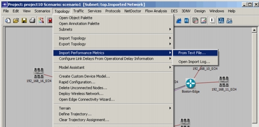
You can apply performance metrics information from a text file over a cloud model, using the menu option Topology > Import Performance Metrics > From Text File (highlighted below). This option allows you to import and evaluate operational performance metrics from a comma-separated value (CSV) file. An example of the CSV file is shown in Figure 26.
Figure 24: Import Performance Metrics from Text File
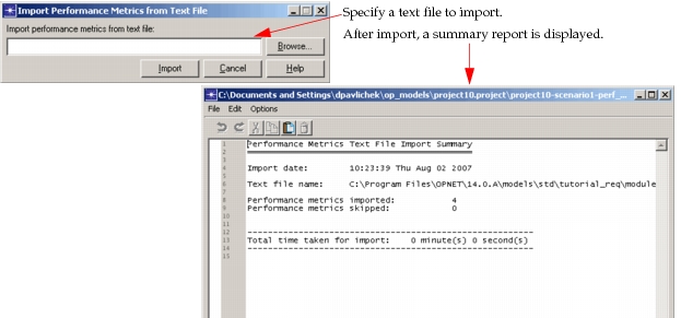
When you select this menu option, a dialog box (shown below) opens, in which you can browse for the text file you want to import. A summary report is displayed after the import to show the metrics that were imported. See Importing Performance Metrics: Example Files for examples.
Figure 25: Import Performance Metrics from Text File Dialog Box and Import Summary
Importing Performance Metrics: Text File Fields
The following fields are supported for the CSV file. Note that while not all fields are required to contain a value, a comma separator must be in place for each field, whether or not a value exists for that field.
Note: The source and destination must be specified—either by using hostnames, IP addresses, or both—in the first four fields.
- Source hostname
- Source IP address
- Destination hostname
- Destination IP address
- Minimum round-trip latency (msecs)
- Maximum round-trip latency (msecs)
- Average round-trip latency (msecs)
- 95th round-trip percentile latency (msecs)
- Minimum source-destination packet loss (%)
- Maximum source-destination packet loss (%)
- Average source-destination packet loss (%)
- 95th percentile source-destination packet loss (%)
- Minimum source-destination jitter (msecs)
- Maximum source-destination jitter (msecs)
- Average source-destination jitter (msecs)
- 95th percentile source-destination jitter (msecs)
Importing Performance Metrics: Example Files
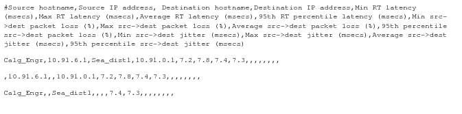
The following figure shows a text file containing the header information (preceded by the # sign) and the values for each field. Note that commas must be present to separate each field, even those with null values. If the text file is not in this format, the performance metrics will not be imported as expected.
Figure 26: Example Text File for Importing Performance Metrics
An example of a performance metrics file, in an Excel file format, is shown below. This example is easier to read and understand. Note that all records contain the IP addresses of the source and destination; some contain the hostnames of the records as well. At least two of the first four fields must be filled in to specify a source and destination pair.
Figure 27: Sample .CSV Performance Metrics File

Importing Performance Metrics: Import Log
The import log is an important source of information for troubleshooting. For each problem encountered during an import, a line is written to the import log. You can select Topology > Import Performance Metrics > Open Import Log... to see an import log dialog box like the one shown below.
Figure 28: Import Log
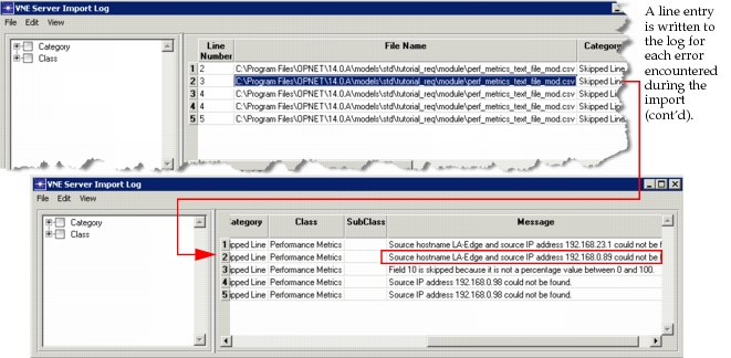
With this information, you can return to the file and make any necessary changes before trying to import the performance metrics again.
Generate Performance Metrics for a Cloud from Router Information
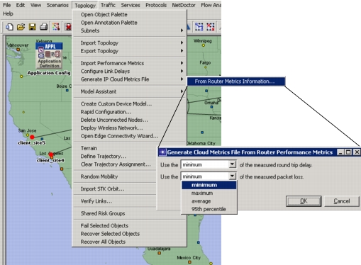
You can also generate performance metrics for a cloud based on router information. In imported networks in which delay and loss metrics have been imported for routers, the performance metrics for the cloud nodes can be determined from the metrics in the router nodes by selecting Topology > Generate IP Cloud Metrics File > From Router Metrics Information…, as shown in the following figure. A new dialog box opens that allows you to specify whether to use the minimum, maximum, average, or 95th percentile of the measured round trip delay and of the measured packet loss specified in the delay, jitter, and loss metrics of the routers.
Figure 29: Generate IP Cloud Metrics from Router Information
The process results in the generation of a performance metrics file for each cloud device in the network. Each file, corresponding to a specific cloud node, contains performance metrics information accumulated from router nodes connected to the cloud node.