PDF Menu Operations
This section contains descriptions and procedures for using the operations available from the PDF menu in the PDF Editor. The items that appear on this menu are described below in alphabetical order:
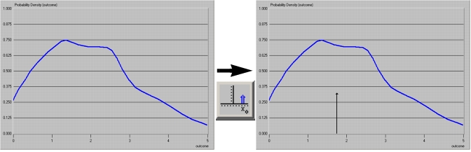
Add Impulse
The Add Impulse operation allows you to add one or more impulses to a probability density function. An impulse is a fixed amount of probability mass associated with a single outcome value. It can be thought of as a sharp, narrow spike in the PDF that gives one particular outcome the specified probability of occurring. More than one impulse can be added to a PDF.
For more information about PDFs, see Chapter 11 "Data Analysis" on page 422.
Figure 226: PDF Before and After Adding an Impulse
Normalize
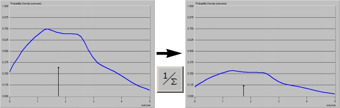
This operation proportionally scales down or scales up a PDF so that the total probability for all outcomes is unity (1).
Figure 227: PDF Before and After Normalizing
Set Abscissa and Ordinate Bounds
The Set Bounds operations modify the upper and lower bounds for the horizontal and vertical axes of a graph.
Figure 228: Using the Set Bounds Operation
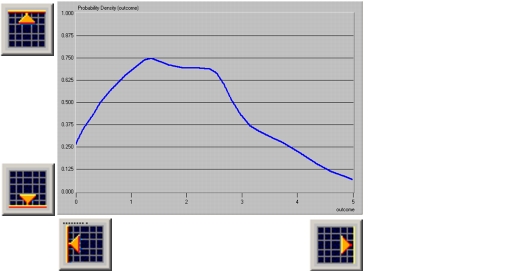
The Set Bounds operations change only the scale and visible portion of an existing graph. The underlying data table—that is, the set of pairs of data points with ordinate/abscissa values—remains unchanged.
Note: Increasing the abscissa range causes a proportional increase in the PDF sample count. A drastic increase in the abscissa range (say, from 5 to 5,000) may cause a memory error. For this reason, a dialog box appears to confirm your choice when entering a bound that more than doubles the current abscissa range.
Set Sampling Resolution
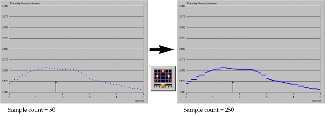
This operation sets the sample count for a graph. The sample count determines how many sample elements, or discrete elements, will be used to approximate a continuous function.
In the context of a PDF, the sample count is the number of discrete outcomes for which a probability weighting is assigned. The default sample count is 500. Based on the user’s graphically-defined PDF, probability weightings are assigned with 500 evenly-spaced outcomes between the low and high bounds of the horizontal axis, inclusive.
The Set Sampling Resolution operation can be used either before a function has been created graphically or after a function has been created or read in. After the sampling count is set, the graph is redrawn at the new resolution.
Figure 229: PDF with Different Resolutions
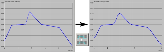
Smooth
This operation rounds out the sharp edges and spikes in a graph. The smoothing algorithm works by sliding a “window” forward along the abscissa of the graph. A dialog box prompts you for the size (in points) of this window; the default setting is three points.
Figure 230: Line Graph Before and After Smoothing