Physical Layer
Packets are transmitted through the air interface, and wireless impairments are considered. Physical layer effects over the transmitted wireless bursts are supported as described in this section. Another purpose of the physical layer implementation is to have a complete configuration of the LTE operational channel to estimate the frame capacity, which is used by the admission control algorithm and the schedulers at the MAC layer of eNodeBs.
The following topics are discussed in this section:
- Frame Structure
- Physical Channels
- Physical Layer Measurements
- Transmission Power
- Uplink Power Control
- Power Consumption Measurement for eNodeB
- Antenna
- Pathloss
- Interference
- Modulation and Block Error Rate
- Multipath Fading
- Multiple-Input/Multiple-Output (MIMO)
- Efficiency Mode
Frame Structure
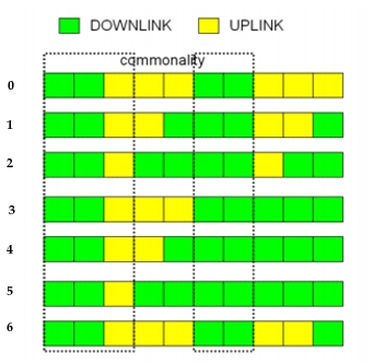
An eNodeB can deploy a physical profile either supporting FDD (Frequency Division Duplex) or TDD (Time Division Duplex) technology. For FDD, both uplink and downlink need their own spectra for operation, while for TDD, uplink and downlink share the same radio spectrum. The TDD mode provides 7 different configurations to divide the radio resources between uplink and downlink to support asymmetric traffic requirements, and can result in better usage of resources due to its flexibility (see Table 144).
The following parameters define the frame structure, the duplexing scheme, and the operational spectrum:
Fixed Parameters
Frame Structure Type: Type 1
- Frame Length: 10 ms
- Subframe length:1 ms
- Slot length: 0.5 ms
Frequency Domain
- A resource block consists of 12 sub-carriers, each 15 kHz wide. The length of a resource block is one slot.
- A resource element is a tile that is one symbol wide and one sub-carrier high. Therefore a resource block has 84 or 72 resource elements depending on the configured cyclic prefix length.
- A pair of two Resource Blocks (RBs) is the minimum allocation unit used by the scheduler while determining the allocations on a frame. The pairing is in time domain, making the allocation unit one subframe (1 ms) in length.
- Downlink reference symbols occupy four resource elements in each RB of the downlink channel. This overhead is accounted for while computing the frame capacity for the admission control procedure.
- Uplink reference symbols occupy 12 resource elements in each RB of the uplink channel. This overhead is accounted for while computing the frame capacity for the admission control procedure.
Configurable Parameters on LTE Config Node
Duplexing Scheme – Both Frequency Division Duplex (FDD) and Time Division Duplex (TDD) are modeled. FDD Profiles are configured under LTE PHY Profiles > FDD Profiles and TDD Profiles are configured under LTE PHY Profiles > TDD Profiles.
FDD/TDD Parameters
Bandwidth – Allowed values are 1.4, 3.0, 5.0, 10.0, 15.0, and 20.0 MHz. For FDD profiles, this is configurable under FDD Profiles > UL SC-FDMA Channel Configuration > Bandwidth for uplink and FDD Profiles > DL OFDMA Channel Configuration > Bandwidth for downlink. For TDD profiles, this is configurable under TDD Profiles > TDD Channel Configuration > Bandwidth. The respective number of resource blocks NRB is as follows:
Table 143: Channel Bandwidth Parameters¹
| Channel Bandwidth BW_Channel (MHz) | 1.4 | 3 | 5 | 10 | 15 | 20 |
|---|---|---|---|---|---|---|
| N_RB | 6 | 15 | 25 | 50 | 75 | 100 |
Note 1: 3GPP TS 36.101 "User Equipment (UE) radio transmission and reception
Base Frequency – Determines the operational frequency of the channel together with the channel bandwidth. For FDD profiles, this is configurable under FDD Profiles > UL SC-FDMA Channel Configuration > Base Frequency for uplink and FDD Profiles > DL OFDMA Channel Configuration > Base Frequency for downlink. For TDD profiles, this is configurable under TDD Profiles > TDD Channel Configuration > Base Frequency.
Cyclic Prefix Length – Allowed values include normal cyclic prefix and extended cyclic prefix, which result in seven and six symbols per slot, respectively. For FDD profiles, this is configurable under FDD Profiles > UL SC-FDMA Channel Configuration > Cyclic Prefix Length for uplink and FDD Profiles > DL OFDMA Channel Configuration > Cyclic Prefix Length for downlink. For TDD profiles, this is configurable under TDD Profiles > TDD Channel Configuration > Cyclic Prefix Length.
TDD Only Parameters
TDD Channel Index – Determines the "type" of TDD physical profile. Seven types are defined in standard [36.213]. Each type differentiates itself from the others in how the Uplink and Downlink subframes repeat within one frame. This is configurable under TDD Profiles > TDD Channel Configuration > TDD Channel Index.
Table 144: TDD Configurations
| Index | Scheme (Uplink:Downlink) | Downlink % |
|---|---|---|
| 0 | 3:2 | 40 |
| 1 | 2:3 | 60 |
| 2 | 1:4¹ | 80 |
| 3 | 3:7 | 70 |
| 4 | 2:8 | 80 |
| 5 | 1:9 | 90 |
| 6 | 3:3:2:2 | 50 |
Note 1: Default value.
Figure 317: TDD Configurations
Downlink Symbols in Special Subframes – Determines the number of slots used by the Downlink in "special" subframes. A special subframe is a downlink subframe, which is immediately followed by an uplink subframe. This is configurable under TDD Profiles > TDD Channel Configuration > Downlink Symbols in Special Subframes.
As described above, the FDD and TDD physical profiles are specified on the LTE Attribute Config utility node under the group attribute LTE PHY Profiles. Each physical profile is uniquely identified by its name, which is specified under the sub-attribute Name. To deploy a physical profile on an eNodeB, choose the desired physical profile under the attribute LTE > PHY > PHY Profile. All profiles configured on the LTE Attribute Config node will be available for selection.
Physical Channels
The following physical channels are modeled:
-
Primary Broadcast Channel (PBCH) – All messages on this channel are modeled without interference, that is, packet reception is always successful. The following messages are sent on this channel:
- Primary Synchronization Signal (PSS)
- Secondary Synchronization Signal (SSS)
- Master Information Block (MIB)
-
Physical Downlink Shared Channel (PDSCH)
- DL data messages
- System Information Block (SIB)
-
Physical Downlink Control Channel (PDCCH) – Such as downlink L1/L2 control channel
- Transports Downlink Control Information (DCI) messages, which are as follows:
- Allocations for RAR messages
- Allocations for CCCH
- Allocations for unicast uplink and downlink signaling and data messages (from the scheduler)
- While computing the DCI capacity of PDCCH, the overhead of Physical Control Format Indicator Channel (PCFICH) is taken into account
- Transports Downlink Control Information (DCI) messages, which are as follows:
-
Physical Random Access Channel (PRACH)
- Contention-based random access is supported
- The number and format of sequences available in the cell that can be used for the random access preamble transmission is configurable via an eNodeB attribute, and the default is 64. The model assumes that each cell has a distinct set of sequence numbers.
- The number of random access resources available in each frame in the cell is configurable using the corresponding attribute of the eNodeB nodes
- Preamble collisions and contention resolution are modeled
- Random Access Channel parameters can be configured in eNodeB attribute LTE > Random Access Parameters
-
Physical Uplink Shared Channel (PUSCH)
- UL data messages
-
Physical Uplink Control Channel (PUCCH) – Such as uplink L1/L2 control channel
Transmission of scheduling requests (SRs), HARQ ACKs/NACKs, and CQI messages via PUCCH are supported
- PUCCH capacity is configurable via eNodeB's attribute LTE > L1/L2 Control Parameters > PUCCH Configuration
- When a UE attaches to the network, eNodeB grants a PUCCH allocation to the UE, when available, to be used for SR transmissions. UEs that do not obtain an allocation will use RACH to make a scheduling request.
Physical Layer Measurements
Physical layer measurements of SINR are supported for both UL-SCH and DL-SCH. A measurement entity is created for each UE, which records instantaneous values of SINR and smooths them using a measurement window. Thus, the measurement module computes a moving average and the size of the measurement window can be controlled by configuring LTE > Link Adaptation Parameters > Measurement Window Size. For more information about this attribute, see Channel Quality Indicator (CQI) and Link Rate Adaptation.
For the downlink, separate measurements are collected for each subband of the downlink channel, if the scheduler is expected to use Channel Dependent Scheduling (by setting the attribute LTE > Scheduling Mode on the eNodeB as described in Channel Quality Indicator (CQI) and Link Rate Adaptation). No measurements are collected if the simulation is run in the efficiency mode "PHY Disabled".
Note: The measurement entity described above is not listed in or required by the LTE specifications but is part of the Riverbed Modeler modeling design.
Physical layer measurements of RSRP and RSRQ are supported. A measurement entity for RSRP and another for RSRQ is created for each audible eNodeB, thus the UE continuously measures RSRP and RSRQ for all eNodeBs within range in the operating frequency.
Reference signals are not transmitted or received in the model, therefore RSRP and RSRQ measurements are performed on the PSS/SSS signals. Thus, the physical layer updates RSRP and RSRQ every 5ms.
The physical layer also sends indications to the higher layers if the measured RSRQ (averaged over 200ms) violates configured thresholds.
Transmission Power
Maximum transmission power is configurable in watts (W) via the Maximum Transmission Power attribute under LTE > PHY on the UE and eNodeB models.
Maximum power is the transmission power of the device over the entire LTE channel bandwidth. Actual burst transmissions use a transmission power proportional to their assigned fraction of the bandwidth.
Uplink Power Control
LTE uses uplink power control to manage the transmit power of UEs. This way, each UE adjusts its transmit power to an optimal level for achieving the desired received signal quality at its eNodeB while minimizing power consumption and co-channel interference to neighboring cells. The LTE model supports uplink power control for PUSCH and PRACH transmissions, as described in 3GPP’s TS 36.213 and TS 36.321 specifications. UE transmit power is controlled in an open-loop fashion, using estimates of the downlink path loss.
The LTE model allows UEs to periodically report power headroom to the associated eNodeB.
The configuration of uplink power control and power headroom reporting on an eNodeB affects all UEs associated with that eNodeB.
Power Control for PUCSH
Power control for PUCSH transmissions is configured on eNodeB nodes by attributes under LTE > Uplink Power Control Parameters. You can disable power control on PUSCH transmissions by setting the Nominal Power attribute to “Use Max Power”. The default value of nominal power is -50 dBm and the default pathloss compensation coefficient is 0.5 (partial pathloss compensation).
Power Control for PRACH
Power control for PRACH transmissions is configured on eNodeB nodes by attributes under LTE > Random Access Parameters. These attributes are:
- Nominal Power (dBm)
- Preamble Power Ramping Step (dB)
- Msg3 Power Difference (dB)
Power Headroom Reporting
Power headroom reporting is configured on eNodeB nodes by attributes under LTE > Uplink Power Control Parameters > Power Headroom Report Parameters. It is enabled by default.
Power headroom is the difference between computed and maximum transmit power of a UE. When reporting is enabled, each UE computes its power headroom and reports it to the eNodeB, which uses that information to check the feasibility of using the new MCS index determined by link adaptation.
Power Consumption Measurement for eNodeB
Power consumption measurement is supported and is configurable in the following attributes under LTE > PHY on the eNodeB:
- Operating Power – User-specified power consumption rate, in watts (W), of non-transmission activities
- Battery Capacity – User-specified power capacity of the battery for a given device in watt-hours. A value of "Unlimited" may be selected for eNodeB devices that are connected to AC power.
Power consumption includes the total energy consumed by the device for both transmission and non-transmission activities. Power consumption measurement calculates both components and produces a sum at the end of a simulation.
At the end of a simulation, output tables display the results. See Power Consumption Report for more information.
Antenna
- Single-sector eNodeB models use a default gain of 14 dB at boresight
- UE models use a default gain of -1 dB
You can configure the gain via an attribute, LTE > PHY > Antenna Gain (dBi) or by use of the antenna model. For eNodeBs with multiple sectors, only the antenna model can be used, as it describes the directionality of the antenna on each of the sectors.
Pathloss
Relevant pathloss attributes are configurable under LTE > PHY > Pathloss Parameters on the UE nodes.
Note: Certain pathloss models permit additional customization in the Model Arguments sub-attribute; however, many of the pathloss models are fixed.
For information on the pathloss models, as well as shadow fading, see "Pathloss Parameters" on page 7 in the Advanced Wireless Package section of this user guide.
Interference
The interference model is supported as follows:
- Interference module detects time and frequency overlaps among different bursts
- Interference is proportional to the amount of burst overlap
- Interference may cause burst drops for PUSCH and PDSCH bursts
- Interference effects for control channels are based on a probability distribution function.
- PUCCH, PDCCH, and PHICH may carry different control signals. Errors in the transmission of those signals are based on uniform distribution functions with configurable average values for each type of control signal (e.g., SR, HARQ-ACK, UL-DCI, DL-DCI, and so on) under LTE > L1/L2 Control Parameters on eNodeB.
- Interference is computed among nodes using the same or different LTE PHY profiles
- The frequency attributes of a given LTE PHY profile are accounted for computing interference
- Interference among different cells (e.g., eNodeBs) can be reduced or eliminated by assigning different LTE PHY profiles with non-overlapping frequency bands to each cell
- Burst representation
- PUSCH and PDSCH assumes contiguous resource block allocations for each individual burst (e.g., per UE)
- PUSCH burst duration is one subframe
- PDSCH burst lasts from the end of PDCCH until end of subframe
Modeling Interference Using Jammer Nodes
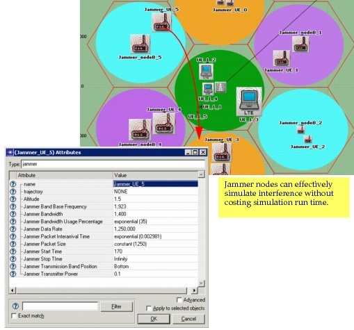
LTE nodes are compatible with jammer node models. Packet transmissions from a jammer node can interfere with the reception of LTE packets. With jammer nodes, you can realize the effect of interference due to adjacent cells, other wireless technologies or a malicious node. By using jammer nodes instead of LTE nodes to model co-channel interference due to adjacent cells, you can realize the following benefits:
- Reduce simulation time and memory
- Reduce model configuration time (versus configuring many individual nodes)
When should I use a jammer node model?
The use of single band jammer node is especially recommended when you are trying to model co-channel interference from adjacent cells (see "Single-Band Jammer" on page 340). The attributes in a single band jammer model can be configured such that the jammer packet transmissions are similar to the transmission from adjacent interfering UEs or eNodeBs.
Note: To see an example of an LTE network that is configured with jammer node models, open the LTE example project and view the "video_perf_under_coch_interference_w_jammers" scenario.
How is the transmission time of a jammer packet configured?
The transmission time of a jammer packet is equal to the value of the Jammer Packet Size attribute divided by the value of the Jammer Data Rate attribute. Usually, LTE transmissions (UL or DL) last for a subframe. To configure a jammer node model to cause co-channel interference as if it were another LTE node, configure Jammer Packet Size and Jammer Data Rate attributes such that the duration of a jammer packet is equal to one LTE subframe (1 millisecond).
How is the frequency band of a jammer packet configured?
The frequency band of a jammer packet transmission depends on the values of the "Jammer Band Base Frequency", "Jammer Bandwidth", "Bandwidth Usage Percentage", and "Transmission Band Position" attributes.
- In FDD, UL and DL subframes are usually configured to operate with different base frequencies, although the total bandwidth is generally the same.
- In TDD, UL and DL subframes operate with the same base frequencies and total bandwidth.
Key Concept— Note the Base Frequency and Bandwidth from the FDD (UL or DL) or TDD profile, and set them in the jammer node model, as depicted in the example shown in Figure 318.
The example shown below provides guidance for configuring the jammer node model. Note that the attributes work synergistically to create the interference you wish to model.
Figure 318: Example Jammer Node Configuration
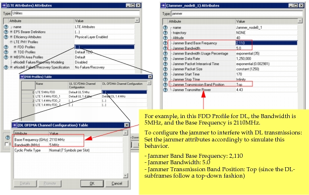
Some attributes are further described below. For more information, see "Single-Band Jammer" on page 340 in the Wireless Module User Guide.
Jammer Bandwidth Usage Percentage
In a typical cellular communication system, such as LTE, the entire bandwidth is not always in use; rather, it exhibits random peaks and valleys. When using jammer node models to model interference due to a neighbor UE or eNodeB, you can set the "Jammer Bandwidth Usage Percentage" to reflect a realistic percentage of bandwidth utilized by jammer packet transmissions.
Note: Although you can select "Full Bandwidth" as an option, it is not recommended when a jammer node is used to model interference due to a neighbor UE or eNodeB. Use a distribution instead, to model realistic behavior.
Jammer Transmission Band Position
Allows you to configure where exactly the jammer packet should be in the frequency axis.
- In UL subframes, the frequency assignment is performed in a bottom-up fashion. Therefore, when trying to interfere with UL subframes, it is preferable to introduce the jammer packet at the "Bottom" of the transmission band.
- In DL subframes, the frequency assignment is in either a top-down or a bottom-up fashion. Therefore, when trying to interfere with DL subframes, it is preferable to introduce the jammer packet at the "Top or Bottom" of the transmission band.
- For TDD, since there is a mixture of top or bottom, you can also optionally set to "Top or Bottom" setting.
- If you use the "Random" setting, the minimum frequency of the jammer packet transmissions can be anywhere between the Jammer Base Frequency and Jammer Base Frequency + Jammer Bandwidth.
For a thorough explanation and illustration of this concept for the jammer model, see "Jammer Bandwidth Band Position" on page 341 in the Wireless Module User Guide.
The following figure shows a typical LTE model with single-band jammers configured to model interference.
Figure 319: Jammer Nodes in LTE Model
Modulation and Block Error Rate
Modulation and Coding Scheme
The Modulation and Coding Scheme (MCS) Index is configurable via the LTE > PHY > Modulation and Coding Scheme Index attribute on UE nodes and remains fixed during the entire simulation. This attribute does not affect the simulation when the LTE > Scheduling Mode attribute on the eNodeB is set to "Link Adaptation Only" or "Link Adaptation and Channel Dependent Scheduling". In each of these cases, the MCS index is dynamically changed based on the link adaptation procedure.
Modulation Curves
Modulation curves plotting the signal-to-noise ratio (SNR) versus block error rate (BLER) are available for all modulation and coding indices except for modulation and coding index 6. Convolutional turbo coding with circular rate matching algorithm are implemented in obtaining the modulation curves.
The modulation curves pertaining to LTE are available in the LTE models directory, <reldir>\models\std\lte, and are name as follows, depending on function, where <x> refers to the modulation and coding index number:
lte_mcs<x>_bler.md.m– Common to uplink and downlinklte_mcs<x>_dl_bler.md.m– Downlink onlylte_mcs<x>_ul_bler.md.m– Uplink only
The modulation curves can be viewed using the Modulation Curve editor, as described in the following procedure.
Procedure 76: View Modulation Curves
- Choose File > Open in the Project Editor.
- Select Modulation Curve from the drop-down menu.
- Select the modulation curve model.
- Click OK to view the selected modulation curve.
End of Procedure 76
Multipath Fading
The model supports ITU Multipath Channel models Pedestrian A, Pedestrian B, Vehicular A, and Vehicular B. You can add more multipath channel models in the LTE configuration node under the attribute "Multipath Channel Definitions".
Selecting Multipath Fading Definitions in the UE
The Multipath Channel Model is selectable on each UE in the following attributes:
- LTE > PHY > Multipath Channel Model (Downlink) and
- LTE > PHY > Multipath Channel Model (Uplink)
By default, LTE OFDMA ITU Pedestrian B and LTE SCFDMA ITU Pedestrian B multipath channel models are configured, respectively.
Defining the Multipath Channel Models
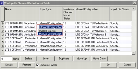
You can define multipath channels in the LTE configuration utility node that can be selected on each UE node, as described above. You can either specify the multipath parameters manually or import the parameters from a file.
Figure 320: Setting Multipath Parameters on the LTE Config Node
Key Concept— If you create a directory containing custom files (for example, custom probability matrixes or Signal-to-Noise [SNR] mapping functions), you must add this directory to the model directories (mod_dirs) in Riverbed Modeler.
Custom probability matrix files and SNR mapping files must be formatted according to the supported type. For example, "mpath_tpm" (Transition Probability Matrix) or "mpath_snr" prefixes must be used in the file names, respectively. These files are text files with the extension gdf, which contain comma-separated values to indicate each row in the transition probability matrix or the coefficients of each polynomial for the SNR translation functions.
To see an example, look at the input files provided in the following location:
<reldir>\models\std\wireless\wrls_phy_mpath_data_files.
Multiple-Input/Multiple-Output (MIMO)
Two antenna models are supported in LTE: single-input/single-output (SISO) and MIMO. SISO systems permit only one antenna at the transmitter and one antenna at the receiver, while MIMO systems permit multiple antennas to be used, as described in this section.
The model supports MIMO in the following ways:
Antenna Diversity
MIMO Antenna Diversity is supported on both uplink and downlink. Antenna diversity reduces the effect of multipath fading on the SNR of the received signal. Therefore, to use this feature, multipath fading must be enabled.
The following attribute on the eNodeB lets you configure the MIMO method to be used in the downlink. To use antenna diversity in the downlink, Transmit Diversity (default) must be selected.
- LTE > MIMO Transmission Technique
The following attributes on the eNodeB and the UE let you configure the number of transmit and receive antennas.
- PHY > Number of Transmit Antennas
- PHY > Number of Receive Antennas
The following diversity configurations are supported:
Table 145: MIMO Antenna Diversity
| Antenna Configuration (Transmit x Receive) | ||||||||
|---|---|---|---|---|---|---|---|---|
| 1x2 | 1x4 | 2x1 | 2x2 | 2x4 | 4x1 | 4x2 | 4x4 | |
| Downlink | ✓ | ✓ | ✓ | ✓ | ✓ | ✓ | ✓ | ✓ |
| Uplink | ✓ | ✓ |
By default, the eNodeB supports two transmit antennas and two receive antennas, and the UE supports one transmit antenna and two receive antennas.
Spatial Multiplexing
Open Loop Spatial Multiplexing using Large Delay CDD (Cyclic Delay Diversity) is supported on the downlink only. Multi-codeword spatial multiplexing used in LTE effectively increases the capacity of downlink transmissions by allowing two simultaneous codeword (MPDU) transmissions, which have the same time and frequency information. The codewords are transmitted by one downlink HARQ process. Two ACK/NACK bits, one per codeword, are transmitted by the UE for acknowledgement purposes.
The following spatial multiplexing configurations are supported:
Table 146: Supported MIMO Spatial Multiplexing Configurations
| MIMO Transmission Technique | Transmit Antennas (eNodeB) | Receive Antennas (UE) |
|---|---|---|
| 2 Codewords - 2 Layers | 2 | 2 |
| 2 Codewords - 3 Layers | 4 | 4 |
| 2 Codewords - 4 Layers | 4 | 4 |
The following attributes on the eNodeB and the UE let you configure the number of transmit and receive antennas.
- LTE > PHY > Number of Receive Antennas
- LTE > PHY > Number of Transmit Antennas
To enable spatial multiplexing in the cell, one of the spatial multiplexing modes must be selected from the following eNodeB attribute.
- LTE > MIMO Transmission Technique
Note: The MIMO Transmission Technique attribute can also be configured on the UE nodes. For UEs that prefer to use their own settings rather than what is configured in their serving cells, the MIMO Transmission Technique attribute must be set on the UE.
Note: If a UE does not have the minimum required number of receive antennas to support spatial multiplexing (see Table 146), the eNodeB will use antenna diversity instead when communicating with the UE.
Note the following.
- When MIMO spatial multiplexing is used with the efficiency mode set to "Efficiency Enabled" on the LTE configuration node, only the increase in downlink subframe capacity will be modeled.
- When MIMO spatial multiplexing is used with the efficiency mode set to "Physical Layer Enabled" on the configuration node, both the increase in downlink subframe capacity and the physical layer effects of using MIMO spatial multiplexing will be modeled. However, multipath fading must be enabled on the UE to realize the physical layer effects accurately.
Note: The physical layer effects of using spatial multiplexing may increase the block error rate and therefore the drop probability of a packet at the physical layer.
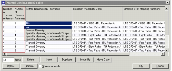
Each multipath channel definition (shown in Figure 320) is composed of a set of multipath channel models for different MIMO combinations. In the attribute table where these individual channel models are defined, you can also specify the corresponding number of transmit and receive antennas and the MIMO Transmission Technique (highlighted in the figure below) for each of the multipath channel models.
Figure 321: MIMO Antenna Diversity Configuration for Multipath Fading
Efficiency Mode
Efficiency mode can be enabled and configured in the LTE configuration node under the attribute "Efficiency Attributes". Efficiency attributes control the mode in which the simulation is run.
- If set to Physical Layer Enabled, each packet goes through wireless pipelines, and all physical layer effects are simulated. This increases accuracy at the cost of simulation speed.
- If set to Efficiency Enabled, packets are directly delivered to the recipient. This mode is useful when the expected average frame drop probability is already known. You can tune various related attributes to cause random packet drops and make the simulation as realistic as possible. In this mode
- Simulation run-times are decreased
- Data frame drops are based on probability distributions (e.g., instead of detailed collision detection)
- Features based on PHY layer modeling (such as Link Adaptation and Channel Dependent Scheduling) are not available