Viewing Attenuation Along a Path
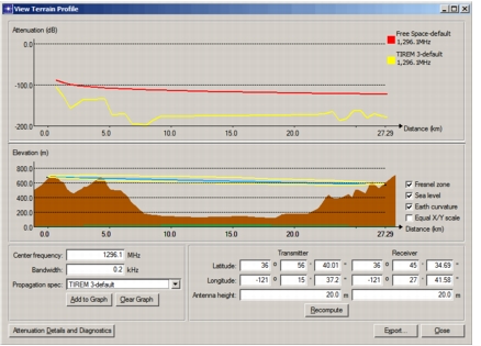
Attenuation traces show path loss at various points between a transmitter and receiver. They are drawn on the upper graph in the View Terrain Profile dialog box, as shown in Figure 14. Each point on an attenuation trace represents the path loss in decibels for a receiver at the corresponding distance from the transmitter (attenuation at the transmitter is 0 dB and is not shown). You can export data representing the terrain profile and attenuation traces to a spreadsheet for further analysis.
The Add to Graph button allows you to add one or more attenuation plots to the View Terrain Profile dialog box. You can create a family of plots, each for a different combination of frequency, bandwidth, and propagation specification.
Procedure 14: Viewing an Attenuation Plot
-
If one is not open, open a View Terrain Profile dialog box showing the signal path of interest, as described in Procedure 13.
-
From the pull-down menus, select the propagation specification to use for the path loss calculations.
If you want to define a new propagation specification for the calculations, refer to Creating a Propagation Specification.
-
Click the Add to Graph button to generate the attenuation plot.
To see an attenuation table and any messages generated by the path loss calculations, click the Attenuation Details and Diagnostics button.
-
To add additional plots to the graph, change the configuration as desired (for example, different frequency or propagation specification) and click the Add to Graph button.
-
If desired, click the Export… button to send terrain profile and attenuation data to a spreadsheet.
Figure 14: Attenuation Graph with Two Plots