3D Network Visualizer
3D Network Visualizer (3DNV) functionality lets you create three-dimensional animations based on topology information, node relationships, performance statistics, and terrain data. You can, for example, use 3DNV to visualize network characteristics such as node placement, line-of-sight restrictions, transmission quality, throughput, delay, and message status information.
This tutorial provides a quick introduction to 3DNV. It shows how you can use 3DNV to do the following tasks:
- Prepare a model for 3D animation.
- View 3D animation of a network model in the Riverbed Modeler workspace (planning mode).
- View 3D animation of a simulation in progress (simulation mode).
- Save and replay a 3D animation.
Before You Begin
To do this tutorial, you must have the following licenses available:
- Riverbed Modeler
- 3D Network Visualizer GUI
- Terrain Modeling Module
- Wireless
- Discrete Event Simulation
Note that, because OpenFlight terrain is not supported on Linux, you can do this tutorial only on Windows platforms.
You should have the following software and hardware installed on your computer:
- Riverbed Modeler 18.6
- 3D Network Visualizer 3.2.0
- 3DNV Communications 3.2.0 (must be installed on every computer running either Riverbed Modeler or 3DNV)
- 128-bit video card with at least 256MB of video memory and support for OpenGL 2.1 or later
This tutorial assumes you have a basic knowledge of how to use Riverbed Modeler to configure nodes and run simulations.
Note: If you have problems with any of the 3DNV programs during this tutorial, see Troubleshooting at the end of this tutorial.
Configuring Riverbed Modeler
Before beginning this tutorial, you must configure Riverbed Modeler by setting three preference values.
Procedure 1: Configuring Riverbed Modeler
-
Start Riverbed Modeler.
-
Choose Edit > Preferences…
Result: The Preferences dialog box opens.
-
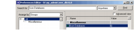
The 3DNV tutorial network uses custom icons. Set the Icon Databases preference to specify their location, as follows:
-
3.1 Type Icon Databases in the Search box.
Figure 1: Preferences Dialog Box with Search Box Entry

-
3.2 Press <Enter> or click the Find button.
Figure 2: Preferences Dialog Box with Preference Located
-
3.3 Click in the Value cell of the Icon Databases preference.
Result: The Icon Databases dialog box opens.
-
3.4 Select the <empty> row.
-
3.5 Click the Insert button, type wireless_corps, and press <Enter> to accept the value.
-
3.6 Click OK to accept the changes and to close the Icon Databases dialog box.
-
-
The 3DNV tutorial uses custom node models. Set Modeler to recompile models by removing any references to existing model repositories:
- 4.1 Type Network Sim in the Search box and press <Enter>.
- 4.2 If the Network Simulation Repositories preference value is not (), click in the Value cell, delete all repository names, and close the Network Simulation Repositories dialog box.
-
The 3DNV tutorial uses the same terrain database in Riverbed Modeler and 3D Network Visualizer. To ensure that 3D positions are in synch between the two programs, Riverbed Modeler needs to use an ellipsoid representation of Earth similar to the one used in 3D Network Visualizer. This replaces the default spherical model (which is faster to compute):
- 5.1 Type Earth in the Search box and press <Enter>.
- 5.2 If the Earth Geocentric Model preference value is not ellipsoid, click in the Value cell and choose ellipsoid.
-
Click OK to close the Preferences dialog box.
Result: A dialog box appears indicating that the Earth Geocentric Model and Icon Databases preferences require the tool to be restarted for the changes to be taken into account. Click OK to dismiss this dialog box.
-
Quit and restart Modeler to make the icons available and to use the ellipsoid earth model.
Using Multiple Computers
The 3DNV module can be installed on the computer running Modeler or on a different computer. A different computer (as shown in the following figure) is recommended for best performance.
Figure 3: Running Modeler and 3DNV on Separate Computers
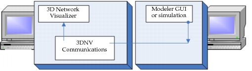
If Modeler and 3DNV are installed on different computers, you must configure the installation in two ways. (If they are on the same computer, skip these steps and go to the Introduction.) First, edit the rid.mtl file on both computers.
Procedure 2: Configuring for Multiple Computers
-
Use the installation CD to install 3DNV_RTI_3.2.0 (the 3DNV Communications program) on the computer running Modeler.
Note: The RTI was installed on the 3DNV computer as part of the 3DNV installation.
-
On the Modeler computer, use a text editor to open the file <install_dir>\3DNV\3.2.0\configs\rid.mtl, where <install_dir> is the path to the software (for example, C:\OPNET).
-
Confirm that the file contains the following line:
(setqb RTI_tcpForwarderAddr "<ip_addr>")where <ip_addr> is the IP address of the other computer (on which the 3DNV Communications program will be run).
-
If necessary, add or edit the line and save the file.
-
Repeat steps 2–4 on the 3DNV computer, verifying that the line exists and has the IP address of the 3DNV computer.
When this tutorial asks you to run 3DNV programs (for example, 3DNV Communications and 3D Network Visualizer), run them on one computer and Modeler on the other.
Introduction
The 3DNV_Tutorial network consists of 20 mobile MANET nodes located in the vicinity of Monterey, California. These nodes are clustered in four groups representing tanks, troop carriers, airplanes, and helicopters.
Figure 4: 3DNV_Tutorial Network
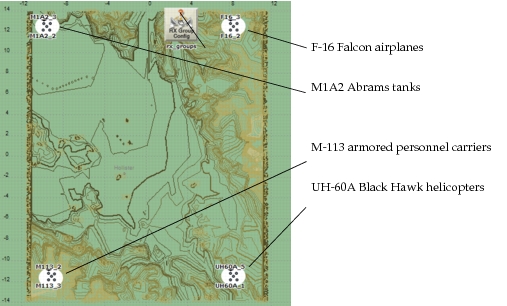
During the course of a simulation, each group of nodes follows a trajectory across the terrain, converging on a point near the center of the map. As they move, the nodes communicate with each other—initially with other nodes of the same group and then with other groups as they get closer.
3D Animation Architecture
Modeler and 3DNV work together as members of an HLA federation. HLA (High-Level Architecture) is a protocol that allows two or more programs to exchange data and run in time-step together.
Figure 5: Sample 3D Animation Federation

There are three parts to the federation used to display 3D animation.
Table 1: Parts of a 3D Animation Federation
| Part | Purpose | Program |
|---|---|---|
| Data generator | Produce animation data | Modeler GUI, simulation process, or Multi-Federate Logger for 3DNV |
| Run-time infrastructure (RTI) | Moderate communications within the federation | 3DNV Communications |
| One or more data receivers | Display or record the animation data | 3D Network Visualizer or Multi-Federate Logger for 3DNV |
3DNV and Modeler work together as members of an HLA federation.
Preparing a Model for 3D Animation
Before you can view 3D animation of a network model, you must configure the model to work with 3DNV. There are two basic requirements:
-
The network model must have a terrain database specified.
-
The nodes to be animated must be mapped to specific shapes (called entities in 3DNV) using a 3DNV mapping library.
(In this tutorial, we use the default mapping library, which relies on the 3DNV Mapping attribute definition discussed later.)
Typically, you will also assign trajectories to mobile nodes, so that their movement can be visualized. This is not a requirement for using 3DNV, however.
Animation with 3DNV requires a network model with a terrain database and nodes mapped to 3DNV entities.
You'll begin this tutorial by modifying a sample network model to specify a terrain database, add the necessary attribute, and map the nodes to the appropriate 3DNV entities.
The network model uses an elevation map of the Monterey region. A matching terrain database must be specified. You will specify a terrain database in OpenFlight format, which is the preferred type for 3DNV.
Procedure 3: Specifying a Terrain Database
-
Start Modeler, if it is not already running.
-
Choose File > Open…
-
In the file browser, go to the <reldir>\models\std\tutorial_req\module\3dnv directory, where <reldir> is the path to the software (for example, C:\Riverbed\18.6). Then open the 3dnv_tutorial project.
Result: The 3dnv_tutorial network (baseline scenario) opens in the Project Editor.
-
Choose File > Save As… and save the project in your default model directory as <your_initials>_3dnv_tutorial.
-
Choose Topology > Terrain > Manage Terrain Specifications…
Result: The Manage Terrain Specifications dialog box opens.
-
Click the Create New Terrain Specification… button, enter a name <your_initials>_3dnv_terrain, and click OK.
-
Select the Global Default checkbox for your terrain specification.
-
Specify a terrain source for your terrain specification:
-
8.1 Click the Add Source… button.
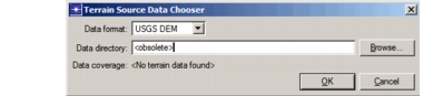
Result: The Terrain Source Data Chooser dialog box opens.
Figure 6: Terrain Source Data Chooser
-
8.2 In the Data format pull-down menu, select OpenFlight.
-
8.3 Click the Browse… button and use the file browser to choose the file <reldir>\models\std\tutorial_req\module\3dnv\N36_45_0W121_30_0.flt.
Result: The geographic limits of the terrain data are displayed in the “Data coverage” field.
-
8.4 Click OK.
Result: The terrain source is added to the Data Sources list.
-
-
Click the Apply Changes and Close button to save the terrain specification.
To display sites (nodes and subnets) properly in 3D Network Visualizer, Modeler must know how to map each one to a 3D entity model that 3D Network Visualizer can display. This is done by assigning a value to the 3DNV Mapping attribute on each site to be animated. 3DNV is shipped with a default mapping library that uses the value of this attribute to determine how to map node and subnet instances to 3D entities.
In most cases, you will need to add the 3DNV Mapping attribute to each site to be displayed. A public attribute definition named 3DNV_Mapping comes with Modeler. You can use this definition to add the 3DNV Mapping attribute to most node models and to node and subnet instances.
You will now add a 3DNV Mapping extended attribute to each of the mobile nodes in the model. You could do this by modifying the underlying node model, but this requires Riverbed Modeler and the ability to freely change node models that might be shared by many users. Also, although a single node model is used in this tutorial, it is much simpler to add an extended attribute to a set of nodes without having to modify all of their models.
Procedure 4: Adding and Configuring the 3DNV Mapping Extended Attribute on Each Mobile Node
-
Choose 3DNV > Manage 3DNV Entities…
Result: The Manage 3DNV Entities and Associated Visualizations dialog box opens.
Figure 7: Manage 3DNV Entities and Associated Visualizations Dialog Box
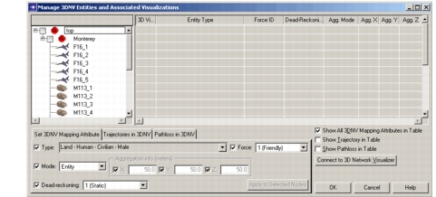
Each node has a corresponding row in the table to the right. Because none of the nodes have a 3DNV Mapping attribute yet, no values are shown in the table.
-
Select the five F16 nodes in the tree.
-
Under the Set 3DNV Mapping Attribute tab, choose Air - Plane - F-16 Falcon from the Type pull-down menu.
-
Click the Apply to Selected Nodes button.
Result: A 3DNV Mapping extended attribute is added to each of the selected nodes, with values based on the selected fields on the Set 3DNV Mapping Attribute page.
Figure 8: Planes with 3DNV Mapping Attribute Added
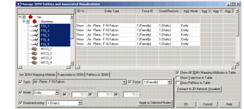
Result: The F16 nodes will now look like F-16s in the 3DNV animation.
-
Repeat steps 2–4 to set the mapping of the remaining mobile nodes, as follows:
- M113 nodes – set Type to Land - Vehicle - M113 Armored Personnel Carrier
- M1A2 nodes – set Type to Land - Vehicle - M1A2 Abrams
- UH60A nodes – set Type to Air - Helicopter - UH-60A Black Hawk
-
Click OK to commit the changes to the modified nodes.
The network model is now configured for use with 3D Network Visualizer. Save it and continue with the tutorial.
-
Choose File > Save.
Viewing 3D Animation in Planning Mode
When you have a network model that is configured for 3D animation, you can use 3DNV to examine the placement of nodes in the surrounding terrain and to visualize movement along trajectories. The mode in which you view animations of the GUI workspace is called planning mode.
Planning mode lets you visualize node placement and movement from the workspace, without running a simulation.
Viewing Node Placement
First, open project and scenario that has been configured for 3D animation. Then start the 3D animation software, select a terrain database for the animation background, and start communications between Modeler and 3D Network Visualizer.
Procedure 5: Opening the Project and Starting the 3D Animation Software
-
If necessary, open the project <your_initials>_3dnv_tutorial. Make sure the current scenario is baseline.
-
In Windows, choose Start > Programs > OPNET 3D Network Visualizer 3.2.0 > OPNET 3DNV Communications 3.2.0.
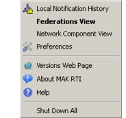
Result: 3DNV Communications is the RTI that controls the transfer of data from Modeler to 3DNV. It starts with no window. Instead, you should see an icon in the notification area of the Windows taskbar. You can right-click on that icon to view information about the HLA Federation.
Figure 9: RTI Icon

Figure 10: Pop-Up Menu for RTI Icon
-
In Windows, choose Start > Programs > OPNET 3D Network Visualizer 3.2.0 > OPNET 3D Network Visualizer 3.2.0 (1.3, 32 Bit).
Note: The (1.3, 32 Bit) part of the program name specifies the RTI type and the bitness of the program. You can choose the (1.3, 64 Bit) version if your computer supports it.
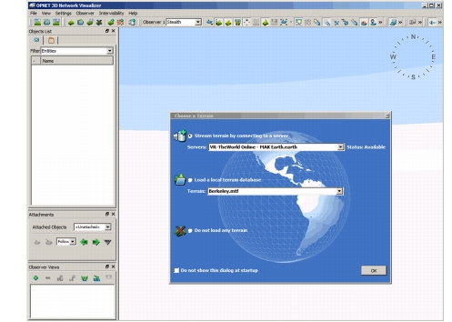
Result: After a short delay, the 3D Network Visualizer window and the Choose a Terrain dialog box open (Figure 11).
Figure 11: Initial 3D Network Visualizer Window
-
Select the Load a local terrain database radio button, then select Monterey.mtf from the pull-down menu and click OK.
Note: If the Choose a Terrain dialog box does not open, choose File > Open Terrain…, select Monterey.mtf, and click Open.
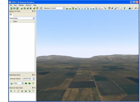
Result: The Monterey.mtf file specifies various types of information needed by 3D Network Visualizer and references the same terrain database specified earlier in Modeler. 3D Network Visualizer loads and displays the terrain.
Figure 12: 3D Network Visualizer Window with Terrain Loaded
-
In Modeler, choose 3DNV > Display 3D Network View.
Result: A checkmark appears in front of the Display 3D Network View menu item, showing that it is enabled. Modeler establishes communications with 3D Network Visualizer and shares information about the network.
Now you can select the node you want to watch in the animation. For this tutorial, we'll follow one of the Black Hawk helicopters.
Procedure 6: Selecting the Node to Watch for the Animation
-
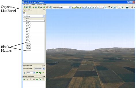
In 3D Network Visualizer, look at the Objects List Panel on the left-hand side of the window.
Note: If the panel is not open, choose View >Objects List Panel to display it.
Result: You will see a treeview listing all of the nodes in the connected model.
Figure 13: Objects List Panel
-
Right-click on the first Black Hawk object (UH60A_1) in the Objects List Panel and choose Attach Tether in the pop-up menu.
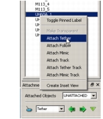
Result: The view mode is now tethered to the UH60A_1 object and will follow that object if it moves. The entity name and view mode are listed in the Attachment Panel.
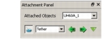
You can now see UH60A_1 in the 3D Network Visualizer window. It looks like a helicopter, as specified by the DIS Entity Type attribute of the 3DNV Mapping compound attribute (Air - Helicopter - UH-60A Black Hawk).
Figure 14: UH60A_1 in 3D Network Visualizer Window
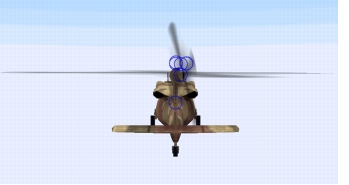
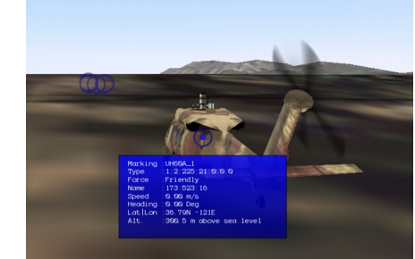
You should see a large blue circle in the center of the Black Hawk model, as well as several others on the horizon. Each circle represents the location of an entity and can be used to view information and perform right-click operations as in the Objects List Panel.
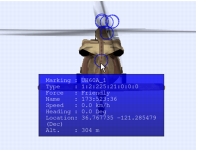
If you move the cursor over the helicopter's blue circle, you will see information about the entity.
Figure 15: UH60A_1 Entity Information
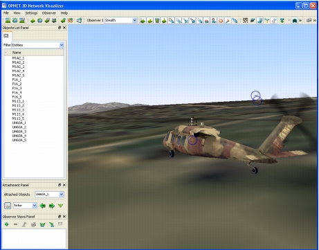
You can rotate the view around the associated tethered entity with the arrow keys. For example, press the left-arrow key a few times to rotate the view to the right and you'll see two of the other Black Hawks.
Figure 16: Rotated View
Press the space bar to reset the viewpoint to its default position (in the case of Tether, this is behind the entity, looking “ahead”).
You can use planning mode to help place nodes at desired points in the terrain. As you move a node in the Modeler workspace, the animation view changes correspondingly.
Procedure 7: Placing a Node
-
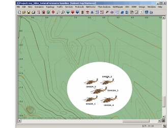
In Modeler, zoom in on the Black Hawk group and some of the surrounding terrain.
-
Find UH60A_1 and drag it to a new location in the workspace.
Result: The node moves in the 3D Network Visualizer window and the surrounding landscape changes accordingly.
-
Drag UH60A_4 to a position close to directly “above” the UH60A_1 icon.
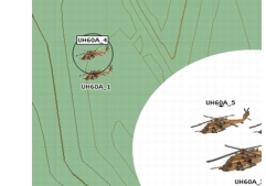
Result: You will see several blue circles near UH60A_4. These represent the positions of other nodes in the model. You can move the cursor near or over a circle to display information about that object.
Viewing Node Movement
Planning mode is also useful for visualizing the trajectories of mobile nodes. 3DNV lets you see the relative positions of multiple nodes as they move.
To see this, you must first add trajectories to the mobile nodes by editing their Trajectory attributes. To save time here, you will use a scenario pre-configured with four different trajectories.
Procedure 8: Adding Trajectories to the Mobile Nodes
-
In Modeler, choose 3DNV > Display 3D Network View.
Result: This toggles 3D display off. The current scenario is disconnected from 3DNV and all node objects disappear from the 3D Network Visualizer window.
-
Choose Scenarios > Switch To Scenario > configured.
Result: A scenario that has been pre-configured with mobile node trajectories opens.
-
Connect the new scenario to 3DNV: choose 3DNV > Display 3D Network View.
Result: Modeler reconnects to 3DNV.
-
In the 3D Network Visualizer window, right-click UH60A_4 in the Objects List Panel and select Tether.
To move the nodes automatically, you must use the Modeler time controller. This will step through a specified time range, updating the position of each mobile node at each time step.
Procedure 9: Defining Movement to a Mobile Node
-
In Modeler, choose View > Show Time Controller (or press Ctrl+Alt+T).
Result: The time controller appears.
Figure 17: Time Controller Dialog Box
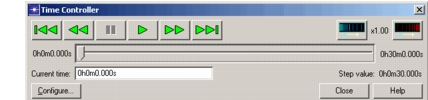
In your networks, you will need to set the time range and step size to useful values. In this tutorial, however, the start and stop times have been preset to match the duration of the mobile node trajectories. The time step needs some adjustment, however.
-
Set the time controller for a smaller time step, to produce smoother-looking animation:
-
2.1 In the time controller, click the Configure… button.
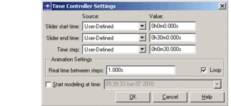
Result: The Time Controller Settings dialog box appears.
Figure 18: Time Controller Settings Dialog Box
-
2.2 Change the time step value to 5 seconds (0h0m5.000s).
-
2.3 Notice that the Loop checkbox is selected. This will cause the time controller to loop repeatedly through the specified time range.
-
2.4 Click OK to close the Time Controller Settings dialog box.
-
-
In the time controller, click the Play button.
Result: The time controller steps through its time range. At each time step, node positions are updated in the Modeler workspace and 3D Network Visualizer shows the node movement between positions.
-
In the time controller, click the Pause button to stop the animation.
Moving the Observer
3DNV uses the concept of an observer to represent the position from which you view an animation. Using various keyboard controls, you can move the observer in three-dimensional space and change the direction in which the observer looks. Table 2 lists a few common controls; for a complete set, refer to the “3D Network Visualizer Quick Reference Card”.
Table 2: Common Observer Movement Keys
| Movement Function | Key |
|---|---|
| Move forward | w |
| Move back | s |
| Move right | d |
| Move left | a |
| Move up | q, Ctrl + q |
| Move down | e, Ctrl + e |
3DNV lets you view an animation from any location in or around the network terrain. To get a different view of the node movement, change the animation window to look down on the terrain.
Procedure 10: Viewing the Animation from Overhead
-
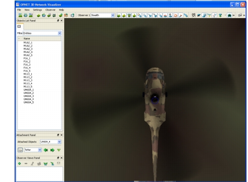
Press the up arrow key repeatedly until you are looking straight down at the helicopter.
-
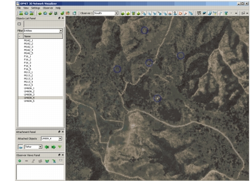
Using the mouse wheel or the “s” key, zoom out until you can see all five helicopters.
-
In the Modeler time controller, click the Play button.
Result: The time controller resumes stepping through its time range and you can see all five helicopters moving over the terrain.
-
Let the animation run for a while, then click the Pause button to stop the animation.
This overhead view will be useful later. 3D Network Visualizer lets you both capture a view for reuse during the current run and also save sets of captured views for use in later runs. A captured view includes the attached object, view mode, observer location, and look direction.
Procedure 11: Capturing and Saving the Overhead View
-
In the Observer Views Panel of the 3D Network Visualizer window, click the Add Current Observer View icon.
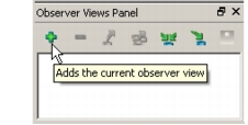
Result: The view is captured and a default name appears in the list.

-
Double-click on the name of the captured view, type Overhead, and press <Enter>.
Result: The view is renamed.
-
In the Observer Views Panel, click on the Export All Views icon.
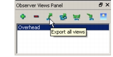
Result: A Save As dialog box opens.
-
Type <your_initials>_views and click Save.
There are many other ways to view an animation. If you want, try moving the observer and look direction for different views of the animation. You can also try some shortcuts. For example:
- Shift + left-click on a node makes that node the attached entity. (Press Space to reset the attach position and orientation for a default view of the entity.)
- Shift + left-click on the terrain teleports to that location. This changes the view to a close-up of that location.
Note: The functions of the navigation controls change in different view modes. If you “lose” the attached node, press Space to return to the default view for the current mode.
One interesting view is to attach to an object and press the left and right arrow keys to orbit around the object.
This ends our look at using 3DNV in planning mode. Perform the following procedure to disconnect the scenario and quit 3DNV.
Procedure 12: Disconnecting the Scenario and Quitting 3DNV
-
In the time controller, click the Close button.
Result: The time controller closes and all nodes return to their starting positions.
-
In Modeler, choose 3DNV > Display 3D Network View to disconnect the scenario.
-
From the 3D Network Visualizer menu bar, choose File > Exit and click Yes in the confirmation dialog box.
-
Right-click on 3DNV Communications 3.2.0 in the Windows task bar and select Shut Down All.
Viewing 3D Animation in Simulation Mode
In addition to viewing node movement and terrain in 3DNV, you can visualize simulation results while a simulation is running. This is called simulation mode. In simulation mode, you can view the following types of simulation data in 3DNV:
- Packet transmission and reception statistics
- Membership of nodes in specific receiver groups
- Successful and failed transmissions
You can use the APIs in the 3D Network Visualizer Package to create custom visualizations of other types of simulation data as well, such as:
- The effect of terrain on wireless communications
- Individual packet transmissions
- Antenna transmission and reception areas for mobile nodes
- Directional networking antenna patterns
- Interference levels for individual frequencies
Simulation mode lets you view a 3D animation showing data generated by a simulation as the simulation runs.
To use simulation mode, you must first configure the network model for 3D animation, as you did in the first part of this tutorial.
Procedure 13: Opening the Project
- If necessary, start Modeler and open the project <initials>_3dnv_tutorial. Make sure the current scenario is configured.
Next, specify the kinds of simulation data to visualize. Modeler provides several utility objects that are pre-configured for certain kinds of simulation data. The utility objects you will use in this tutorial are:
- ovis_anim_comm_lines—generates 3DNV animation visualization of successful and failed packet transmissions by drawing a line between the transmitting and receiving nodes
- ovis_anim_pkstat—generates 3DNV animation visualization of the packet transmission and reception statistics for each node containing transmitters and receivers
- ovis_anim_sim_time_display—generates 3DNV animation visualization of the simulation time
Riverbed Modeler users can develop their own utility objects using the 3DNV API, a extensive collection of functions that support custom 3D animation. You can double-click on these utility objects to drill down to the process model and examine the code used to generate the animation (primarily in the enter execs and header block).
Modeler provides utility objects pre-configured to animate specific kinds of simulation data. Developers can modify these or create their own.
Add some animation utility objects to the network model.
Procedure 14: Adding Animation Utility Objects to the Network Model
-
Click on the Open Object Palette tool button.
Result: The object palette opens.
-
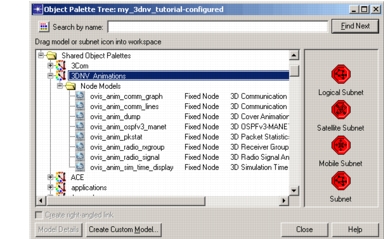
Scroll the palette tree till you see the 3DNV_Animations tree node, then expand that node to display the content of the palette.
Result: A selection of 3DNV utility objects appear in a Node Models tree sub-node.
Figure 19: 3DNV_Animations Object Palette
-
Drag an instance of the ovis_anim_comm_lines object into the workspace near the rx_groups object (the exact location is not important).
-
Right-click on the ovis_anim_comm_lines object, select Edit Attributes, and set the following attribute values:
- name –> comm_lines
- Transmission Line Color –> green
Click OK to close the Attributes dialog box.
-
Drag an instance of the ovis_anim_pkstat object into the workspace and set its attributes as follows:
- name –> pk_stats
- Reception Statistic Color –> white
- Transmission Statistic Color –> white
Click OK to close the Attributes dialog box.
-
Drag an instance of the ovis_anim_sim_time_display object into the workspace and set its attributes as follows:
- name –> sim_time
- Color –> yellow
Click OK to close the Attributes dialog box.
-
Close the object palette.
-
Save your changes to the model.
Next, start the 3D animation software and prepare it to receive animation data from a simulation.
Procedure 15: Starting the 3D Animation Software
- In Windows, choose Start > Programs > OPNET 3D Network Visualizer 3.2.0 > 3DNV Communications 3.2.0.
- In Windows, choose Start > Programs > OPNET 3D Network Visualizer 3.2.0 > OPNET 3D Network Visualizer 3.2.0.
- From the 3D Network Visualizer menu bar, choose File > Open > Terrain…
- Select Monterey.mtf and click Open.
Now prepare the Modeler simulation to send animation data to 3DNV.
Procedure 16: Preparing the Simulation to Send Animation Data to 3DNV
-
In Modeler, choose DES > Configure/Run Discrete Event Simulation (or click the “running man” button).
Result: The Configure/Run DES dialog box appears.
-
Make sure the Use OPNET Simulation Debugger (ODB) checkbox is not selected.
-
In the treeview, select Inputs > Terrain Modeling.
Result: The dialog box displays the Terrain Modeling tabbed page.
-
Select the Use Terrain Modeling Module checkbox.
-
Select the Use custom settings radio button.
-
From the Propagation specification pull-down menu, select Longley Rice-default.
-
From the Terrain specification pull-down menu, select <your_initials>_3dnv_terrain.
-
In the treeview, select Outputs > Animation > 3D.
Result: The dialog box displays the 3D animation tabbed page.
-
Select the Use 3DNV Module checkbox.
Result: This tells the simulation to generate 3DNV data. The other 3DNV controls become enabled.
One of these controls is Record history in file with an appropriately-named file. All 3DNV data generated by the simulation via Ovis APIs will be recorded in this file for later playback. This is independent of actually sending live 3DNV updates to the 3D Network Visualizer during the simulation. This allows you to replay the 3DNV visualization afterwards from the graphical environment.
-
Select the Live output via 3DNV Communication checkbox.
Result: This tells the simulation to send generated animation data directly to the 3D Network Visualizer.
-
In the treeview, select Execution > Advanced > Kernel Preferences.
Result: The dialog box displays the Kernel Preferences tabbed page.
-
In the Real-time execution ratio field, enter 5.
Result: This tells the simulation to run at up to five times real-time speed. In other words, the simulation will pace events so that the run takes about 6 minutes of clock time (30 minutes of simulation time divided by the real-time ratio of 5).
Finally, run the simulation and view the animation in 3D Network Visualizer.
Note: If the simulation and 3D Network Visualizer are running on the same computer, they might run quite slowly. Typically, you should either run Modeler and 3D Network Visualizer on different computers or capture the simulation output and replay it in 3D Network Visualizer later (as you will do in the next part of this tutorial).
For best results, quit all programs on your computer except those needed by this tutorial.
Procedure 17: Running the Simulation
-
In the Configure/Run DES dialog box, click the Run button.
Result: The simulation starts up.
After a delay, the simulation connects to 3DNV. (The delay will be longer the first time the simulation is run, while Modeler compiles some of the models.)
-
After the node list appears, right-click on UH60A_3 in the Objects List Panel and select Attach Tether.
Result: The selected object appears in the 3D Network Visualizer window. The simulation data you specified also appears, as shown in the following figure.
Figure 20: Visualization Showing Simulation Data
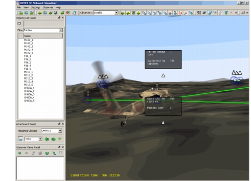
Packet statistics for an object appear in associated text boxes around the entity. To avoid an overly crowded and confusing display, these text boxes are not shown initially. Instead, they are represented by small triangles near each entity. Moving the cursor inside one of these triangles will display the information for that entity. Clicking on a triangle toggles between displaying the information permanently or only when the cursor is inside the triangle.
Note: You might need to use the left or right arrow keys to rotate the view to separate UH60A_3’s information triangle from those of other entities.
Green lines connect transmitting and receiving nodes to show successful communications. Red lines represent failed communications.
The simulation time appears in the lower-left corner of the window. The simulation time is updated when a packet is transmitted or received.
Note: Updates to the animation display occur only when animation events are generated by the simulation; for example, when packet broadcasts force node position updates. As a result, updates occur at irregular intervals and the animation can appear “choppy” at times.
-
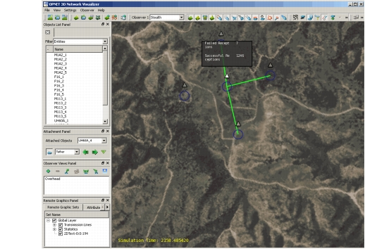
After watching the animation for a while, you can switch to the overhead view you saved; this provides a better view of the communication lines:
-
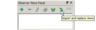
3.1 From the Observer Views Panel, click the Import and Replace Views icon.
-
3.2 Select <your_initials>_views.osrx in the file list and click Open.
Result: The saved view appears in the Observer Views Panel.
-
3.3 Click Overhead in the View List.
Result: The animation changes to the overhead view you saved earlier, showing UH60A_3 and near-by objects.
Figure 21: Visualization Showing Simulation Data—Overhead View
-
-
When the simulation completes:
- 4.1 In the Simulation Sequence dialog box, click the Close button.
- 4.2 In Modeler, choose File > Save.
- 4.3 From the 3D Network Visualizer menu bar, choose File > Exit and click Yes in the confirmation dialog box.
Replaying 3D Animation
During the simulation all the 3DNV outputs were recorded in a 3DNV history file, as well as sent out to the 3D Network Visualizer. The recorded history can be played back later to show part or all of the 3D visualization.
Now you can play back the recorded animation and view it in 3D Network Visualizer.
Procedure 18: Replaying the 3D Animation
-
In Windows, choose Start > Programs > OPNET 3D Network Visualizer 3.2.0 > OPNET 3D Network Visualizer 3.2.0.
-
From the 3D Network Visualizer menu bar, choose File > Open > Terrain…
-
Select Monterey.mtf and click Open.
-
In the Project Editor, choose 3DNV > Play 3DNV History…
Result: A file browser opens.
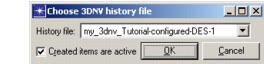
Figure 22: Choose 3DNV History File
-
Verify that the listed file matches the current scenario and click OK.
Result: The 3DNV History playback dialog box appears.
Figure 23: 3DNV History Playback Dialog Box
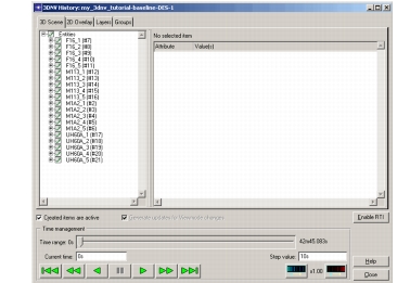
The treeview shows the Ovis entities and decorations that are defined after all operations taking place during events at simulation time 0 have been applied.
At this point, none of the Ovis entities or decorations have been made known to 3D Network Visualizer. When this happens, any object with a checkmark will be made known.
Unchecking items allows you to reduce the amount of traffic sent to 3D Network Visualizer and focus your attention to the items of interest. In this tutorial, let’s focus on the communications between helicopters.
-
Uncheck all of the M1A2 tanks, F-16 planes, and M-113 armored carriers.
-
Click on the Enable RTI button.
Result: This creates appropriate Ovis entities for the five Black Hawk helicopters and their associated entities.
-
After the node list appears, right-click on UH60A_3 in the Objects List Panel and select Attach Tether.
-
Click the Play button.
Result: As the time value increases, the corresponding Ovis changes for checked objects are sent to the 3D Network Visualizer, exactly as happened in simulation mode.
-
At some point, press the Pause button to stop the playback.
Note: After you stop the playback, 3D Network Visualizer will continue to display animation until it catches up to the simulation time at which you paused the playback.
-
Close the 3DNV history playback dialog box.
Result: The Ovis entities and decorations disappear from the 3D Network Visualizer.
-
Close the project, 3D Network Visualizer, and 3DNV Communications.
Troubleshooting
This section provides solutions to some common problems that can occur when using 3D Network Visualizer.
If you have successfully completed this tutorial, skip to Summary.
3D Network Visualizer no longer updates its display when nodes move in Modeler
Communications between Modeler and 3D Network Visualizer time out after a period of disuse. To reestablish communications:
- Disconnect the current scenario from 3DNV (in Modeler, choose 3DNV > Display 3D Network View).
- Quit the 3D Network Visualizer and 3DNV Communications programs.
- Restart the 3DNV programs, as follows:
- a) In Windows, choose Start > Programs > OPNET 3D Network Visualizer 3.2.0 > 3DNV Communications 3.2.0.
- b) In Windows, choose Start > Programs > OPNET 3D Network Visualizer 3.2.0 > OPNET 3D Network Visualizer 3.2.0.
- c) From the 3D Network Visualizer menu bar, choose File > Open > Terrain…
- d) Select Monterey.mtf and click Open.
- Reconnect the Modeler scenario (choose 3DNV > Display 3D Network View).
- Attach an object in 3D Network Visualizer.
While moving the observer, you lose sight of the attached object and can’t find it again
Press Space to reset the view.
Summary
This tutorial has presented a quick introduction to 3DNV. You have seen how to:
- Prepare a model for 3D animation.
- View 3D animation of a network model in the workspace (planning mode).
- View 3D animation of a simulation in progress (simulation mode).
- Save and replay a 3D animation.
For more information about using 3D animation in Modeler, see the Animation Viewers documentation.