Packet Switching I
In this tutorial, you simulate the behavior of a packet switching network. As part of creating the network, you will use the packet and link editors, learn new Kernel Procedures, and define your own statistics.
You will also
- Learn some principles of model design
- Become more familiar with process and node models and how they function in a network model
- Do parametric studies of various statistics
In a simple packet switching network, the performance of the network can be measured by the end-to-end delay experienced by traffic on the network.
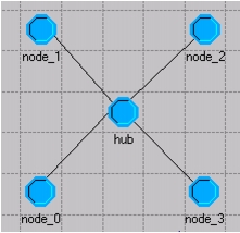
In this lesson, your goal is to model a simple network in which four peripheral nodes generate traffic while a central hub node relays the traffic to the appropriate destination within the network.
Figure 1: A Small Packet Switching Network
Getting Started
There are several design concepts you should consider before you start building the network model:
- Network topology and the physical communication medium
- The functions of the different node types
- The method the process model uses to determine which point-to-point transmitter addresses a particular peripheral node
- The role of peripheral nodes
Network Topology
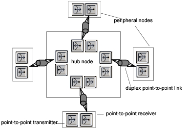
The initial network will consist of four peripheral nodes connected to a hub node by point-to-point links.
Point-to-point links can either be simplex (unidirectional) or duplex (bidirectional). In this case, you will use custom duplex links to connect transmitter-receiver pairs. Looking only at the communications medium as represented, the network would look like the following figure.
Figure 2: Communications Medium of the Network
Functions of the Different Node Types
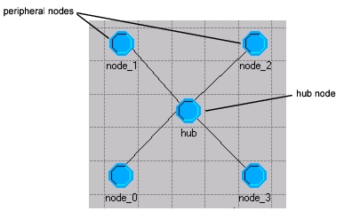
The purpose of the model is to simulate packets traveling from one peripheral node to another peripheral node through the packet switching hub node. In the hub node, you can assume that packets containing destination addresses will arrive randomly on the four incoming links from the four peripheral nodes. The destination address is an integer value specifying a destination peripheral node. The hub node must contain a process model that can retrieve the incoming packets, read the destination address, and send the packets to the appropriate point-to-point transmitter.
Figure 3: Different Node Types
The Role of the Hub Node Model
Packet streams each have a unique index. The easiest method is to set up a direct association between the hub process outgoing packet stream indices and the peripheral destination address values. In a more adaptive model, the hub process model could maintain a table for translating destination address values to transmitter stream indices. In this tutorial, a direct correspondence between designating addresses and packet stream indices is appropriate.
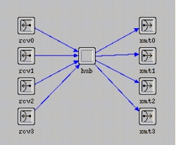
In summary, the hub node model will consist of a point-to-point transmitter/receiver pair for each peripheral node, and a process model used to relay packets from a receiver to the appropriate transmitter.
Figure 4: Hub Node
The Role of Peripheral Nodes
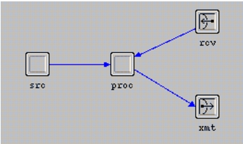
The peripheral node model must generate packets, assign destination addresses, and process received packets. The peripheral node model will use a generator module to create packets. It will use a user-defined process model to assign destination addresses to packets and send them to the node’s point-to-point transmitter. This process model will retrieve packets arriving from the point-to-point receiver. Upon receiving a packet, the same process model will calculate the packet’s end-to-end delay and write the value to a global statistic (a global statistic is accessible to multiple processes throughout the system).
Figure 5: Peripheral Node
Building the Models
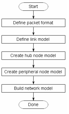
To build this network model, you must do the steps shown in the following figure.
Figure 6: Building the Packet Switching Network
Creating a New Packet Format
The Packet Format Editor can create packets containing any number of different fields that affect packet size.
The packets in this network contain a single field with the destination address of the packet. After the packet format has been created, it can be specified as an attribute in a generator so that packets created by the generator will be formatted accordingly.
Procedure 1: Creating a New Packet
-
If not already running, start the program.
-
Close any open projects.
-
Choose File > New… and select Packet Format from the pull-down list. Click OK.
-
Click on the Create New Field tool button, then move the cursor into the editor window.

-
Left-click to place a field in the editor window, then right-click to end the field creation operation.
Result: A new field is created in the editor window.
Setting the Packet Field Attributes
Procedure 2: Setting the Packet Field Attributes
-
Right-click on the packet field and select Edit Attributes to open its Attributes dialog box.
-
Set the name attribute to dest_address.
-
Make sure the type attribute is set to integer.
-
Set the size attribute to 2. This defines the size of the actual field in bits. For 4 possible addresses, 2 bits is enough.
-
Change the set at creation attribute to unset. This ensures that the field will not be assigned a default value when the packet is created.
-
Click OK when you are finished.
Result: The packet field in the editor window displays its name and field size.

-
Choose File > Save. Name the packet <initials>_pksw_format, then click Save. Close the Packet Format Editor when you are done.
Creating a Link Model
Use the Link Model Editor to create custom links.
Create a link model that connects the hub and peripheral nodes. This duplex link model should support your packet format.
Procedure 3: Creating a Link Model
-
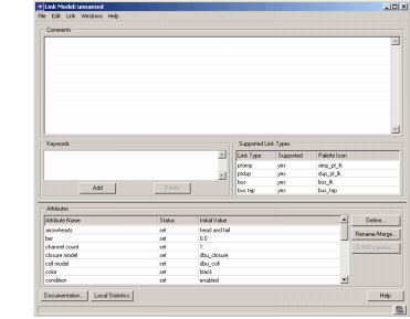
Choose File > New… and select Link Model from the pull-down list. Click OK.
Figure 7: Link Model Editor
Setting the Supported Packet Format
Because the link you are creating supports the packet format you just defined, there are several attributes that must be set.
Procedure 4: Setting the Supported Packet Format
-
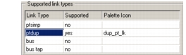
In the Supported link types table, change the value under the Supported field to no for everything except ptdup. The model only needs to support point-to-point duplex.
Figure 8: Link Model Editor (Detail)
-
In the Attributes table, scroll down to the packet formats attribute and click its Initial Value field.
The Select Supported Packet Formats dialog box opens.
-
Unselect the Support all packet formats and Support unformatted packets checkboxes.
-
Change the <initials>_pksw_format packet format’s status value to supported.
-
Click OK to close the dialog box.
Setting Other Attributes
In addition to setting the supported packet format type, you must set the following attributes in the attribute table.
Procedure 5: Setting Other Attributes
- Set the data rate attribute to 9600.
- Set the ecc model to ecc_zero_err (error correction model).
- Set the error model to NONE.
- Set the propdel model to dpt_propdel (point-to-point propagation delay model).
- Change txdel model attribute to dpt_txdel (point-to-point transmission delay).
You might also want to add a comment to the link model to describe it.
Procedure 6: Including the link_delay External File
-
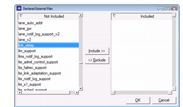
Choose File > Declare External Files…
Result: The Declare External Files dialog box appears.
-
In the Not Included column, look for link_delay.
-
Select the link_delay entry and click Include>>.
-
Click OK to close the dialog box.
-
Choose File > Save, name the link model <initials>_pksw_link, and click Save.
-
Close the Link Model Editor.
Creating the Hub Node
Now that you have defined a packet format and link model to be used in the model, you can create the hub and peripheral nodes. This process requires two steps for each node type: defining the node model and defining the process model.
Start by defining the node model for the hub. The hub needs four sets of transmitters and receivers for incoming and outgoing packets (one set per peripheral node), as well as a central processor to distribute the packets correctly.
Creating the Node Model
Procedure 7: Creating the Node Model
-
Choose File > New… and select Node Model from the pull-down list. Click OK.
-
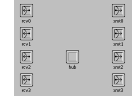
Place a processor, four point-to-point transmitters, and four point-to-point receivers in the editor window as shown in the following figure.
-
Change the name attribute on each object as shown in the following figure.
Figure 9: Hub Node Model
-
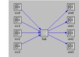
Create packet streams to connect the modules as shown. Start with top transmitter and receiver and work your way down. Be sure to draw the streams from the receivers to the hub, then from the hub to the transmitters.
Figure 10: Hub Node Model Packet Steams
Checking the Packet Stream Assignments
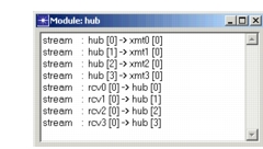
To check the packet stream assignments, do the following.
Procedure 8: Checking the Packet Stream Assignments
-
Right-click on the hub process module and select Show Connectivity from the Object pop-up menu.
Result: The list of streams connecting to the hub module appears.
-
Close the dialog box.
Setting Other Attributes
Now that the hub node model has been created, you need to set the channel data rate and supported packet format for each receiver and transmitter.
Procedure 9: Setting Other Attributes
-
Hold down the Shift key and left-click on each transmitter module icon to select them. Make sure the packet streams are unselected.
-
When all the transmitter modules are selected, right-click on one of the modules and select Edit Attributes to open its Attributes dialog box.
-
Click on the value of the channel attribute. In the (channel) Table dialog box, change the data rate to 9600.
-
Support the <initials>_pksw_format format:
- 4.1 Click on the value of the packet formats attribute.
- 4.2 Unselect both checkboxes to turn off Support all packet formats and Support unformatted packets.
- 4.3 Click on the status field for <initials>_pksw_format and change the status to supported.
- 4.4 Click OK in the Select Supported Packet Formats dialog box.
-
Verify that the correct data rate and packet formats display in the (channel) Table dialog box, then click OK.
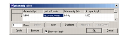
-
To apply changes to all selected objects, click on the Apply changes to selected objects checkbox, then click OK.
If a warning message with information about “undoing” appears on your screen, click Yes to continue.
You should see the text “4 objects changed” in the message area at the bottom of the Node Editor.
-
Left-click in a blank area of the workspace to deselect all modules.
-
Repeat steps 1–7 for the receiver modules. (You cannot update all modules at once because transmitter and receiver channels have different attributes.)
Setting Interfaces
The last step to defining the hub node module is to specify that only fixed node types are supported
Procedure 10: Setting Interfaces
-
Choose Interfaces > Node Interfaces.
-
In the Node types table, change the Supported value to no for both mobile and satellite node types.
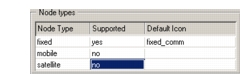
-
Optionally, add a comment to describe the node. When you are finished, click OK to close the dialog box.
The hub node model is now complete, except for specifying the process model for the hub processor module (which you can do once the process model has been created). For now, save the model as <initials>_pksw_hub, BUT DO NOT CLOSE IT.
Creating the Process Model of the Hub Node
In this model, the hub receives a packet and, based on the destination address, forwards it to the correct transmitter, which sends it to the destination node.
Now, create the hub process model.
In your node model, the hub processor module is connected to the transmitters and receivers by packet streams. Because each packet is associated with an interrupt, the hub process model receives an interrupt whenever a packet arrives from a receiver. Because this is the only expected type of interrupt, the hub process FSM (finite state machine) can be defined using one unforced idle state to rest between events and a transition executive containing the code for processing packets.
Procedure 11: Creating the Process Model of the Hub
-
Choose File > New… and select Process Model from the pull-down list. Click OK.
Result: The Process Editor Startup Wizard opens.
-
Click Quit in the Wizard to start with an empty model.
-
Using the Create State tool button, place one state in the editor window.
-
Change the name attribute of the state to idle.
-
Use the Create Transition tool button to draw a transition from the idle state to itself.
-
Right-click on the transition and select Edit Attributes. Change the condition attribute to PK_ARRVL and the executive attribute to route_pk().
When a packet arrives from a point-to-point receiver, the process model is invoked by a stream interrupt. The transition must test for this condition.
-
Click OK to close the attribute dialog box for the transition.
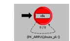
-
Define the PK_ARRVL macro:
-
8.1 Click on the Edit Header Block tool button.

-
8.2 Enter the following macro definition for PK_ARRVL:
#define PK_ARRVL (op_intrpt_type () == OPC_INTRPT_STRM) -
8.3 Choose File > Commit and then File > Close when you are finished.
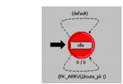
The PK_ARRVL condition compares the delivered interrupt type with the predefined symbolic constant OPC_INTRPT_STRM, which indicates a stream interrupt. Although this is the only expected type of interrupt for this model, it is good to safeguard against run-time missing transition errors. To do this, you can create a default transition loop on unforced states.
-
-
Create a default transition on the unforced state:
-
9.1 Create a transition from the idle state back to itself.
-
9.2 Change the condition attribute to default and click OK to close the dialog box.
You also must define the route_pk() transition executive.
-
9.3 Click on the Edit Function Block tool button.
-
9.4 Enter the following code:
static void route_pk(void) { int dest_address; Packet * pkptr; FIN(route_pk()); pkptr = op_pk_get(op_intrpt_strm ()); op_pk_nfd_get_int32 (pkptr, "dest_address", &dest_address); op_pk_send (pkptr, dest_address); FOUT; } -
9.5 Choose File > Commit and then File > Close when you are finished.
This code executes when the FSM follows the transition.
-
The first line after FIN(route_pk()) has two effects: first, it retrieves the arriving packet from the appropriate input stream (whose index is determined by op_intrpt_strm()). Then, op_pk_get() uses the packet-stream index argument to return a pointer to the packet.
Next, the process must obtain the destination address contained in the packet. The destination address is held in the packet’s dest_address field, which is an integer data type. The second line of code assigns the destination address to the dest_address local variable.
Remember that the destination address corresponds directly to the outgoing packet stream index of the hub node. The final line of code sends the packet to the correct point-to-point transmitter based on the destination address.
Finally, you can define the model interface attributes for the process and compile the model. First, enable the begsim intrpt attribute, as described in the following procedure.
Procedure 12: Defining the Model Interface Attributes
- Choose Interfaces > Process Interfaces.
- Set the begsim intrpt attribute to enabled.
- Add a comment if you want, then click OK when you are finished with the Process Interfaces.
Now, compile the process model.
Procedure 13: Compiling the Model
-
Click on the Compile Process Model tool button.

-
Name the file <initials>_pksw_hub_proc, then click Save.
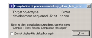
Result: The compilation status dialog box appears.
-
When the Status changes to done, click Close.
-
Choose File > Close to close the Process Editor.
After you define the hub process model, you can set the process model attribute of the hub processor module in the Node Editor.
Procedure 14: Assigning the Process Model to the Node
-
Choose Windows > Node Model > <initials>_pksw_hub.
Result: The Node Model Editor window becomes active.
-
Right-click on the hub module and select Edit Attributes. Change the process model attribute to <initials>_pksw_hub_proc.
-
Click OK to close the Attributes dialog box.
-
Save the node model.
Creating the Peripheral Node Model
When a peripheral node generates a packet, it must assign a destination address to the packet, then transmit it to the hub. When it receives a packet, the node must record the packet’s end-to-end delay. To accomplish these tasks, a peripheral node model must consist of a generator module, a processor module, and a point-to-point transmitter and receiver.
Procedure 15: Creating the Peripheral Node Model
-
Make sure you have saved your hub model, then choose Edit > Clear Model.
Result: The workspace is cleared. This avoids the step of closing and reopening the Node Editor.
-
Save As… <initials>_pksw_node to save the model you are about to construct.
-
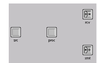
Place and name the modules as shown the following figure.
-
Create packet streams to connect the different modules in the following order:
- rcv to proc
- proc to xmt
- src to proc
Verify the assignment of packet streams between the modules. Right-click on the proc module and choose Show Connectivity from the pop-up menu to see the following table.
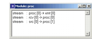
If the streams are not correct, the simulation might not generate results. If necessary, correct the streams by deleting all links and recreating them as specified in above.
After creating the network models, you want to run simulations for different packet interarrival times, setting the Packet Interarrival Time attribute just before running the simulations. To make it possible to set the attribute then, you need to promote the attribute. To do this, you need to edit the attributes of the src module.
-
Right-click on the src module to open its Attributes dialog box.
-
Change the process model attribute to simple_source.
-
Click on Packet Interarrival Time in the left column to highlight the Attribute name, then right-click and select Promote Attribute to Higher Level from the pop-up menu.
Result: The Packet Interarrival Time attribute is promoted so that its value can be set later.
We also want the processor to create packets with the previously-defined format.
-
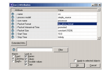
Specify <initials>_pksw_format as the value for the Packet Format attribute.
-
Verify that your (src) Attributes table is similar to the one in the following figure, then click OK.
Next, we want to change the data rate and supported packet formats for the receiver and transmitter. You did this same operation earlier, in the hub module.
-
Make sure the packet streams are unselected. This could happen when you select the first receiver.
-
Right-click on the transmitter module and select Edit Attributes.
-
Click on the value of the channel attribute. In the (channel) Table dialog box, set the data rate (bps) to 9600.
-
Support the <initials>_pksw_format format, as follows:
- 13.1 Click on the value of the packet formats attribute.
- 13.2 Unselect both checkboxes to turn off Support all packet formats and Support unformatted packets.
- 13.3 Click on the status field for <initials>_pksw_format.
- 13.4 Click OK to close the Select Supported Packet Formats dialog box.
-
Verify that the correct data rate and packet formats display in the (channel) Table dialog box, then click OK.
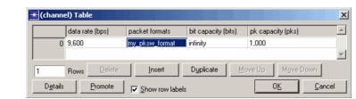
-
In the open Attributes dialog box, click OK.
Result: The message “1 object changed” appears in the status bar. 16. Repeat steps 11–15 for the receiver module.
The next step in defining the peripheral node model is to specify that only fixed node types are supported. You did this same operation earlier, in the hub module.
Because the node is fixed, not mobile or satellite, you need to edit the model attribute interfaces. 17. Choose Interfaces > Node Interfaces. 18. In the Node types table, change the Supported value for mobile and satellite types to no, and add a comment to describe the model, if you want. 19. Do not close the Node Interfaces dialog box. You still need to use it.
Renaming attributes allows you to simplify complex attribute names or to expand terse ones.
You might want to simplify attribute names, especially when long hierarchical names are confusing and unnecessary. You might also want to expand a highly-abbreviated attribute name to make it more understandable.
For this model, you will rename the interarrival time attribute. 20. In the Node Interfaces dialog box, click on the Rename/Merge… button. 21. In the Unmodified Attributes pane, select the src.Packet Interarrival Time attribute, then click on the >> button to move it to the Modified Attributes pane. 22. Change the text in the Promotion Name column to source interarrival time.

- Click OK to close the Rename/Merge Attributes dialog box.
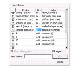
You can assign a set of symbolic values to an attribute to provide a simpler user interface. Your assigned values are displayed as options in a list.
There are several advantages to assigning symbolic names to attribute values:
- Options can be limited to appropriate values.
- Options can be assigned descriptive names, making it easier for a user to select the correct value.
- Users can select values from a list, avoiding typographical errors.
Add symbolic values to the source interarrival time attribute: 24. In the Attributes table of the Node Interfaces dialog box, select the newly-renamed source interarrival time attribute, then click on the Edit Properties… button.
Result: The Attribute: source interarrival time dialog box appears. 25. In the Symbol map table, change the status of all symbols to suppress by clicking in the status column of each row. 26. Add entries in the Symbol map as shown, then click OK to close the dialog box.
Hiding attributes simplifies an interface. This is desirable when the end user does not need to change an attribute value. Hiding an attribute does not affect its value during simulation.
Many attributes that appear in the peripheral node are not relevant to this model. To avoid confusion and clutter, these attributes can be hidden. 27. In the Attributes table of the Node Interfaces dialog box, change the status of all attributes except source interarrival time to hidden.
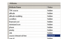
- Click OK to close the Node Interfaces dialog box.
- Choose File > Save to save the model.
Creating the Process Model of the Peripheral Node
The peripheral node process model does two main functions:
- assigns destination addresses and sends packets
- keeps track of end-to-end delay
To complete its tasks, the peripheral node process model needs two states:
- an initial state
- an idle state
Procedure 16: Creating the Process Model of the Peripheral Node
-
Choose File > New… and select Process Model from the pull-down list. Click OK.
Result: The Process Editor Startup Wizard opens.
-
Click Quit in the Wizard to start with an empty model.
-
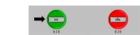
Put two states in the editor window as follows:
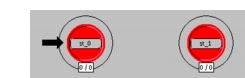
-
Change the attributes of the states, as indicated:
-
4.1 For the initial state, change the name attribute to init and the status to forced.
-
4.2 For the other state, change the name attribute to idle. (Leave the status as unforced.)
In the init state, the process model will load a uniform PDF in a range of 0 to 3.
Next, create transitions between the states in the process model:
-
-
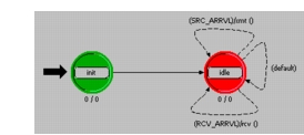
Draw the transitions between the states and specify the transition conditions and executives as shown in the following figure.
The xmt() transition executive will generate and assign destination addresses to packets as they arrive from a generator. Packets will then be sent on to the point-to-point transmitter.
The rcv() transition executive is entered when a packet arrives. In the executive, the process model will determine the packet’s end-to-end delay, update the global statistic, and destroy the packets.
-
Next, click on the Edit Header Block tool button to define the transition macros for SRC_ARRVL and RCV_ARRVL in the header block.

-
Enter the following code:
/* packet stream definitions */
#define RCV_IN_STRM 0
#define SRC_IN_STRM 1
#define XMT_OUT_STRM 0
/* transition macros */ #define SRC_ARRVL (ev_type == OPC_INTRPT_STRM && ev_strm == SRC_IN_STRM) #define RCV_ARRVL (ev_type == OPC_INTRPT_STRM && ev_strm == RCV_IN_STRM)Note the use of constant definitions of stream indices (
RCV_IN_STRM,SRC_IN_STRM, andXMT_OUT_STRM) for easier code interpretation. The stream indices correspond to the values set in the node model.ev_typeandev_strmare two variables that will be set in the exit executives of the idle state before these transition conditions are evaluated. -
Choose File > Commit and then File > Close when finished.
Next, you need to define the end-to-end delay statistic that will be collected when each packet arrives at its destination.
-
Choose Interfaces > Global Statistics.
-
Enter the Stat Name as ETE Delay.
-
Click in the Description column and enter the following text in the dialog box:
Calculates ETE delay by subtracting packet creation time from current simulation time. -
Choose File > Commit to accept and close the dialog box.
-
Verify that the completed Declare Global Statistics dialog box looks like the following figure.

-
Close the Declare Global Statistics dialog box by clicking on the OK button.
Finally, you need to add the executives for some states and transitions in the process model. First add the enter execs for the init state, as described in the following steps. 15. Double-click on the top half of the init state to open its enter execs, then enter the following code:
```
address_dist = op_dist_load ("uniform_int", 0, 3);
ete_gsh = op_stat_reg ("ETE Delay",
      OPC_STAT_INDEX_NONE, OPC_STAT_GLOBAL);
```
- Choose File > Commit and then File > Close.
Temporary variables are meaningful between the exit executive of an unforced state and the enter executive of the subsequent unforced state. They are useful to extract information to use in transition conditions to avoid repeating code.
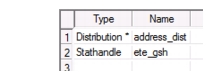
Define the state and temporary variables, as described in the following steps. 17. Define the state variables:
-
17.1 Click on the Edit State Variables tool button.

-
17.2 Enter the following information in the table:
-
17.3 Click OK when you are finished with the state variables.
- Define the temporary variables:
-
18.1 Click on the Edit Temporary Variable tool button.

-
18.2 Enter the following variable definitions:
int ev_type, ev_strm; -
18.3 Choose File > Commit and the File > Close when finished.
In this example, both transition conditions rely on the interrupt type and (in the case of a stream interrupt) the stream. So, instead of obtaining these twice, it’s better to obtain them once in the exit executives of the idle state. 19. Add code to set values for the temporary variables:
-
19.1 Double-click on the bottom half of the idle state to open its exit execs, then enter the following code:
ev_type = op_intrpt_type(); if (ev_type == OPC_INTRPT_STRM) ev_strm = op_intrpt_strm(); -
19.2 Choose File > Commit and the File > Close.
The xmt() transition executive acts when a packet arrives from the generator module. A destination address must be assigned before the packet is sent to the point-to-point transmitter. 20. In the Function Block, enter the following code:
static void xmt(void)
      {
      Packet * pkptr;
      FIN(xmt());
      pkptr = op_pk_get (SRC_IN_STRM);
      op_pk_nfd_set_int32 (pkptr, "dest_address",
         (int)op_dist_outcome (address_dist));
      op_pk_send (pkptr, XMT_OUT_STRM);
      FOUT;
      }
The first statement obtains a pointer to the packet arriving from the generator. The next statement sets the value of the dest_address field, which is an integer data type, to the value returned by the op_dist_outcome() procedure.
op_dist_outcome() returns a random number according to the distribution given as an argument. In this case, address_dist is a pointer to the uniform integer distribution loaded in the init state.
The last statement sends the packet to the output stream, which is connected to the point-to-point transmitter.
The rcv transition executive is entered when a packet arrives on the stream connected to the point-to-point receiver. The purpose of the rcv executive is to calculate and record the end-to-end delay of the packets using a global statistic. 21. In the Function Block, enter the following code:
static void rcv(void)
      {
      Packet *pkptr;
      double ete_delay;
      FIN (rcv());
      pkptr = op_pk_get (RCV_IN_STRM);
      ete_delay = op_sim_time () -
         op_pk_creation_time_get (pkptr);
      op_stat_write (ete_gsh, ete_delay);
      op_pk_destroy (pkptr);
      FOUT;
      }
The first statement in the code after FIN (rcv()) obtains a pointer to the packet arriving from the point-to-point receiver.
The next statement calculates the end-to-end delay by subtracting the packet's creation time from the current simulation time.
The third statement writes the end-to-end delay to a global statistic, and the fourth statement destroys the packet. 22. Choose File > Commit and then File > Close to close the edit pad.
Enable the beginning simulation interrupt. This interrupt starts the process. 23. Choose Interfaces > Process Interfaces. 24. In the Process Interfaces dialog box, change the initial value of the begsim intrpt attribute to enabled.
You may want to add a comment to describe the process. 25. When you are finished, click OK to close the dialog box.
Finally, compile the process model. 26. Click on the Compile Process Model tool button.
 27. Supply the file name <initials>_pksw_nd_proc and click Save.
28. When the process model has finished compiling, close the Compilation dialog box then close the Process Model Editor. (If the model does not compile, check for typographical errors.)
Now that the peripheral node process model is complete, you can update the process model attribute of the proc processor module: 29. If a Node Editor is not already open with the <initials>_pksw_node node model, choose File > Recent Files > Node Model > <initials>_pksw_node. 30. Right-click on the proc module and select Edit Attributes from the Object pop-up menu, then change the process model attribute to <initials>_pksw_nd_proc. 31. Click OK in the Attributes dialog box after you have changed the process model attribute. 32. Save the changes made to the node model, then close the Node Editor.
You are now ready to build the network model.
Building the Network
For the packet switching network, neither the subnet extent nor the grid properties are important.
Now that you have built the underlying node, process, and link models, you can build the network model. Remember that the initial network contains one hub node and four peripheral nodes.
Procedure 17: Building the Network
-
Choose File > New… and select Project from the pull-down list. Click OK.
-
Enter the project name as <initials>_pksw_net, and the scenario name as baseline, then click OK.
-
When the Startup Wizard appears, click Quit. You will specify the scale of the network and a palette manually.
The first thing to do is create an object palette that contains the necessary models.
-
Click on the Open Object Palette tool button.
-
Switch to the icon view by clicking on the button in the upper-left corner of the dialog box.

-
Click on the Configure Palette… button in the object palette.
-
In the Configure Palette dialog box, click on the Clear button, then click on the Node Models button.
-
Include <initials>_pksw_hub and <initials>_pksw_node, then click OK.
-
In the Configure Palette dialog box, click on the Link Models button.
-
Include the <initials>_pksw_link model, then click OK.
-
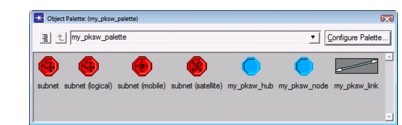
Click OK in the Configure Palette dialog box, name the palette <initials>_pksw_palette, and click Save. If you are using the Wireless module, you will also see mobile and satellite subnet nodes, but your palette should look similar to the following figure.
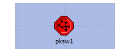
You are now ready to build the network, as described in the following steps. 12. Place a subnet in the editor window and name it pksw1.
-
Double-click on the subnet to move to the subnet view.
-
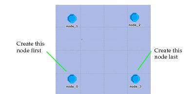
Place four <initials>_pksw_node objects in the window as shown in the following figure.
-
Place one <initials>_pksw_hub in the window, in the middle of the four existing nodes. Name that node hub.
-
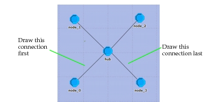
Beginning at node_0, and using <initials>_pksw_link, connect each peripheral node to the hub as shown in the following figure.
Drawing connections in the order node_0. node_1, node_2, and node_3 ensures that your statistics match those shown in this lesson. If you make connections in a different order, your simulation results might differ.
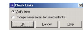
Before you save the project, it is a good idea to get into the habit of checking the links in the network for consistency, ad described in the following steps. 17. Choose Topology > Verify Links (or press Ctrl+L). 18. Make sure that the Verify links radio button is selected, then click OK.
-
If a red X appears over a link, the link is not consistent. In that case:
-
19.1 Choose Topology > Verify Links again.
-
19.2 Select the Choose transceivers for selected links radio button, then click OK.
Result: The red X disappears when the link inconsistency is resolved.
-
For a link to be consistent, the packet formats and data rates of the transmitters and receivers within the objects must match those defined for the link.
Choosing, Collecting, and Analyzing Results
Now that you have built the model, you are ready to simulate network behavior.
To see the effect of the packet generation rate on the performance of the network, you will use two simulation runs with different packet interarrival times.
Choosing Results
Choose the results to be collected during the simulation: end-to-end delay and link utilization.
Procedure 18: Choosing Results
-
Right-click in a blank area of the editor window, then select Choose Individual DES Statistics from the pop-up menu.
-
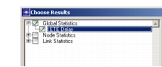
Under Global Statistics, choose ETE Delay. This was the statistic you defined in the peripheral nodes’ process model. When you are finished, click OK.
-
Right-click on the link between node_0 and the hub, then select Choose Individual DES Statistics from the Object pop-up menu.
-
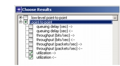
Under point-to-point, choose both utilization statistics. Click OK when you are finished.
-
Save the project with the default name.
Make sure that the repositories preference is set correctly before configuring and running the simulation.
-
Choose Edit > Preferences.
-
Make sure the Network Simulation Repositories preference has the value ().
-
Close the dialog box for the preferences.
Configuring Two Simulation Runs
In this simulation, the source processor creates packets of a constant size. This setting, in combination with the fixed data rate of the point-to-point transmitters and receivers, results in a fixed end-to-end delay for the packets.
However, if packets are sent to a transmitter quickly enough, some of the packets will be delayed in the transmitter’s queue. If the packet interarrival time (source interarrival time attribute) is varied, the end-to-end delay will be affected. To model this, configure two simulation runs with different packet interarrival times.
Procedure 19: Configuring Two Simulation Runs
-
Choose DES > Configure/Run Discrete Event Simulation.
Result: The Configure/Run DES dialog box opens.
Now you will define two simulation runs for two different packet interarrival times. Recall that we promoted the generator’s interarrival time attribute so we could define it now, at simulation time.
To define two simulation runs with packet interarrival times of, respectively, 4 and 40:
-
Change the Duration to 1000 seconds.
-
Change the Seed to 15.
-
Define the interarrival time attribute, as follows:
-
4.1 Click on the Inputs element in the tree.
-
4.2 Click on the Object Attributes element.
-
4.3 Click the Add… button.
-
4.4 In the Add Attribute dialog box, click in the Add? column next to the pksw1.*.source interarrival time attribute and click OK.
-
4.5 In the Configure/Run DES dialog box, click on the newly added attribute name, then click on the Enter Multiple Values… button.
-
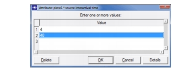
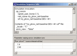
4.6 In the Attribute dialog box, add the Values 4 and 40
-
4.7 Click OK to accept the attribute values.
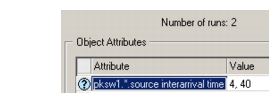
Result: The two values are listed next to the attribute and the total number of runs is now 2.
-
4.8 Click on the Preview Simulation Set button to review how the two runs are set up.
Result: The Simulation Sequence Info dialog box opens, showing the common and per-run information.
-
4.9 Close the Simulation Sequence Info dialog box.
-
-
Click Run to save your changes, close the dialog box, and execute the simulations.
Note: If your computer has multiple cores, you might see a dialog box asking if you want to execute the two runs concurrently. Select the Consecutive Execution checkbox and click Execute Simulations.
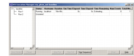
Result: The DES Execution Manager dialog box opens, showing the two configured runs for the baseline scenario. Each simulation run takes a few seconds to run, depending on the speed of your machine.
-
After the simulations complete, close the DES Execution Manager dialog box. If you had problems, see "Troubleshooting Tutorials".
Analyzing Results
To compare the end-to-end delay and utilization between the two simulation runs.
Procedure 20: Analyzing Results
-
Right-click in the Workspace and choose View Results from the pop-up menu.
Result: The Results Browser opens. It lists results for the two runs of the scenario.
-
In the statistics tree, expand:
Object Statistics > pksw1 > node_0 <-> hub[0] > point-to-point and select utilization <--.
Result: Two graphs are shown, corresponding to the two simulation runs for that scenario. You can view the runs in question by expanding the <initial>_pksw_net > baseline tree item.
-
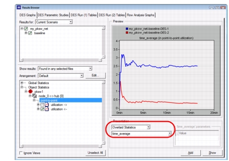
Set the graphing option Overlaid Statistics, then select time_average from the pull-down list of available filters.
-
Click Show.
The time-averaged graph of utilization for this lesson is shown in the following figure.
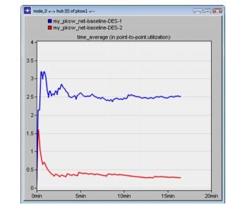
A large reduction in packet generation results in a corresponding reduction in link utilization.
You can change the x-axis to display seconds by right-clicking in the panel (not the graph), then selecting Time Axis > seconds from the pop-up menu.
Close and delete the graph when you are finished.
You also want to look at the end-to-end delay of the packets to see if any queuing occurred.
-
Unselect utilization <-- in the Results Browser dialog box.
-
Expand the Global Statistics statistic tree node, then the ETE Delay node, and finally click <initials>_pksw_net-baseline-DES-1. This allows you to select one data source from the list of available data files.
-
Change the filter type back to As Is, then click Show.
-
Move the graph so that it does not overlap the Results Browser.
-
Unselect <initials>_pksw_net-baseline-DES-1, select <initials>_pksw_net-baseline-DES-2, and finally click Show.
Result: The graphs for end-to-end delay should resemble the ones in the following figure.
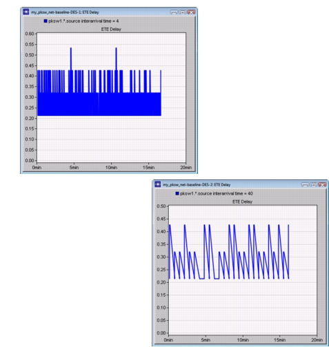
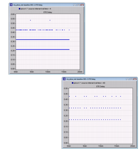
In linear draw style, the graphs do not clearly show the delay experienced by individual packets. To show this, you can change the draw style to discrete.
To change the draw style of one of the ETE delay graphs to discrete:
-
Right-click anywhere in the graph, and choose Draw style > Discrete from the pop-up menu.
Result: The graph changes from a linear to discrete draw style.
-
Perform the same operation for the other ETE Delay graph.
The discrete graphs of ETE delay should resemble those in the following figure.
In the next tutorial, you enhance the current network model by adding a second star network. Return to the list of tutorials in the Contents pane and choose Packet Switching II.