Importing Traffic
This lesson demonstrates traffic import capabilities. In this lesson, you will
- Examine a ready-made model that contains explicit traffic
- Import conversation pair traffic
- Run several simulations to see the effect of traffic growth on the network
In earlier tutorials, you built a network manually by dragging objects from a palette, then you added background load traffic by specifying throughput.
This tutorial shows how to import traffic from external sources. You might import a router configuration file or NetCollector database to create the topology, then import data from different tools, such as NetScout nGenius, Cisco Netflow, or a custom text file to create the traffic.
Reviewing the Ready-Made Model
This tutorial uses a ready-made model with explicit traffic.
Procedure 1: Reviewing the Ready-Made Model
-
Choose File > Open…
- 1.1 The Open dialog box appears.
-
Select Project in the "Files of type" menu (Windows) or Filters menu (Linux). Then navigate to the basic folder using the following path:
<reldir>\models\std\tutorial_req\basic -
Select Imp_Data from the list of files, then click Open.
Result: The network model opens in the workspace.
-
Choose File > Save As…, navigate to your default models directory, and save the project as
<initials>_Imp_Data.There are several types of traffic in Riverbed Modeler:
- Explicitly generated traffic is user-created; you specify the size of the transactions and the number of transactions per time unit according to a chosen distribution. You create explicit traffic by configuring Application Definition and Profile Definition objects.
- Traffic flows (also called conversation pairs or background routed traffic) are special objects that specify end-to-end traffic between source and destination nodes. You can create traffic flows manually using demand objects from the object palette or import them from an external source (Traffic > Import Traffic Flows…).
- Link Baseline Load traffic specifies the background traffic in bits per second. You can create this traffic by configuring the Traffic Information attribute of a link or by importing traffic from various sources using Traffic > Import Baseline Loads.
In this lesson you will use
- Explicitly-generated traffic to test a "what-if" scenario
- End-to-end traffic flows imported from an ASCII traffic archive
To get values for such statistics as delay and response time on a network with background traffic, you must have explicit traffic.
To create explicit traffic (such as an FTP application), you would normally do the following:
- Add and configure Application Definition and Profile Definition objects
- Choose statistics
To run a baseline simulation, you would also need to configure the simulation.
Because you've done these tasks in earlier tutorials, you do not have to repeat them here. The ready-made network model is already configured correctly.
To help you become more familiar with the configuration tasks, we will look briefly at the following:
- Application Definition and Profile Definition objects
- Choose Statistics dialog box
- Configure Discrete Event Simulation dialog box
As a reminder:
- An application definition specifies the applications on the network. For example, Database Access, Email, File Transfer.
- A profile definition specifies the applications used by a particular group of users. A profile definition is applied to a workstation, server, or LAN.
Review the Application Definition and Profile Configuration objects.
-
If you are not already in the 192_9_200 subnet, double-click on it.
-
Specify the applications used in the scenario:
- 6.1 Right-click on the Application Definition configuration object and choose Edit Attributes.
- 6.2 Set the Application Definitions to Default.
- 6.3 Click OK to close the dialog box.
-
In the Profile Configuration object's Edit Attributes dialog box, open the Profile Configuration attribute table by clicking in the Value field and choosing Edit… from the pull-down menu.
-
Verify that the attributes are set as follows:
- Profile Name: FTP (Light)
- Applications: Choose Edit… to display the Applications table, verify that the File Transfer (Light) application is set, then click OK.
- Operation Mode: Serial (Ordered)
- Start Time (seconds): uniform (100, 110)
- Duration (seconds): End of Simulation
- Repeatability: Once at Start Time
-
Click OK to close the Profile Configuration table, then OK to close the Edit Attributes dialog box.
Next, review the statistics specified for collection, as follows.
-
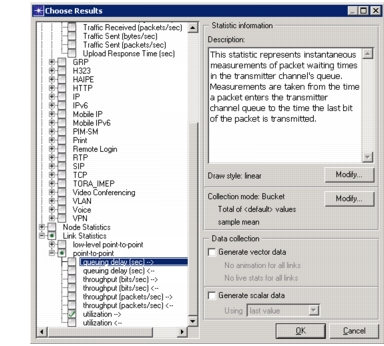
Right-click in the workspace and select Choose Individual DES Statistics from the pop-up menu.
Result: Notice the green dot in the checkboxes next to Global Statistics and Link Statistics. This indicates that statistics in these hierarchies have been chosen for collection.
-
Verify that the following statistics are selected by expanding the hierarchies until you see them, with a green dot in the checkbox.
- Global Statistics > Ftp > Download Response Time (sec)
- Link Statistics > point-to-point > utilization -->
Figure 1: Choose Individual DES Statistics Dialog Box
-
Click OK to close the Choose Results dialog box.
Importing the Traffic Archive
Now that you are familiar with the ready-made model, you can import end-to-end background traffic from a captured traffic archive.
To import a traffic archive, you must do the following:
- Capture or create the traffic. (This has already been done for you.)
- Import the traffic into a scenario.
The following section describes the second step.
Import Procedure
After the traffic archive files have been placed in the correct directory, they can be imported into Riverbed Modeler and applied to the network in the current scenario.
Procedure 2: Importing the Traffic into a Scenario
-
If you are using AppTransaction Xpert and you do not see the Traffic menu in the Project Editor menu bar, do the following:
- 1.1 Choose Edit > Preferences.
- 1.2 In the Search for: field, enter the string aceplus_basic_menus and click Find.
- 1.3 Set this preference to FALSE and then click OK.
- 1.4 If the Traffic menu still does not appear, save the project, restart the program, open the project again, and proceed.
-
Choose Traffic > Import Traffic Flows > From Text (.tr1, .tr2) Files…
Result: The Traffic Import dialog box appears.
-
Click Add Directory… (under the treeview on the left), then select the following directory:
<reldir>\models\std\tutorial_req\basic\traffic(Windows)<reldir>/models/std/tutorial_req/basic/traffic(UNIX)<reldir>describes the directory that contains the current Riverbed Modeler software. To find your<reldir>directory, do the following:- 3.1 Choose Help > About This Application.
- 3.2 Click the Environment tab.
- 3.3 Under System Information, find the Release directory entry.
-
A treeview of directories appears in the upper-left pane. Expand the hierarchy to display the directory where your archive files reside (
<reldir>\models\std\tutorial_req\basic\traffic). -
From the list of available files, select Imp_Data_Traf.tr1.
Probe information appears in the Start and End fields and the file name appears in the Selected archives pane.
Figure 2: Traffic Import Dialog Box
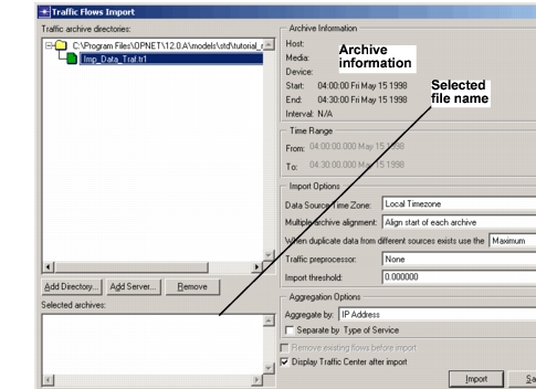
When importing a traffic file, you can specify several different settings, including the time range of the traffic you want to import.
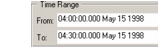
For this lesson, we will use the entire traffic file, which was collected from 04:00–04:30. Note that this time period is set in the From and To options in the Traffic Selection section of the dialog box. You can type different times in the From and To fields if you need to use a subset of the entire traffic collection period.
Figure 3: Selecting the Time Range
When you import traffic from text files, you might need to specify the time zone in which the traffic data was captured. If the traffic file was captured in a different time zone, you can specify the time zone in the Data Source Time Zone field.
Figure 4: Selecting the Time Zone of the Captured Traffic

You can also specify how the import engine handles duplicate traffic. To configure the "traffic merging mode," set the following menu (under Import Options): When duplicate data from different sources exists, use the
<Maximum/Sum/Minimum>.Suppose that you collected data for the following traffic flows at the same time:
- Archive 1 comes from a probe on node 1 that collects traffic sent to node 2
- Archive 2 comes from a probe on node 2 that collects traffic received from node 1
If both probes report the same value, it does not matter if you choose maximum or minimum mode: both modes report the same value. However, if these probes report different values, the specified mode determines which value is used:
- Maximum means the larger amount of traffic is used
- Minimum means the smaller amount of traffic is used
In some cases, the Addition mode is the correct choice. Say, for example, a flow from node 1 to node 2 is split into pieces and sent on multiple paths (one through node A, another through node B).
- If you are collecting traffic only at node 1 or node 2, use either the minimum or maximum mode.
- But if you are, instead, collecting traffic at intermediate nodes A and B, then use the addition mode to correctly consolidate the traffic.
In this case, you will use the most common mode.
-
Set the When duplicate data from different sources exists, use the menu to Maximum.
Figure 5: Selecting the "Traffic Merging Mode"

-
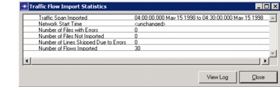
Click Import.
Result: A window appears and shows statistics about the import.
Figure 6: Traffic Flow Import Statistics Window
-
Click Close.
The Traffic Flow Import Statistics window closes and the Traffic Center appears. The Traffic Center enables you to view, analyze, create, and edit all network traffic in one central window.
During import, Riverbed Modeler sometimes cannot associate all imported traffic with the appropriate network objects. This traffic is called unmapped traffic. After an import with unmapped traffic, you have the option to examine the unmapped traffic in the Traffic Center and assign unmapped traffic as needed. Otherwise, if unmapped traffic exists, you can assign it at any time after the import by selecting the Show Unmapped Traffic checkbox in the Traffic Center.
During import, Riverbed Modeler matches imported traffic with endpoints in the network using the node's network alias (usually the node's IP address).
Sometimes Riverbed Modeler cannot match endpoints to network objects for one of the following reasons:
- The node was omitted from the network
- The traffic endpoint is not actually part of the network
In this import, all traffic is matched to an endpoint without a problem. Had a problem occurred, unmapped traffic endpoints can be associated with a network object by selecting the Show Unmapped Traffic checkbox in the Flows Browser and assigning unmapped traffic to specific nodes. For more information about this feature, see "Importing Network Traffic" in the Modeling Concepts manual.
A traffic flow appears as an arrow that connects two nodes, and specifies end-to-end-traffic between those nodes. You can import traffic flows from external programs and files or you can create them manually.
Each traffic flow contains one or more attributes that describe the traffic in that flow.
The model library allows you to create "demand" objects in a network. Traffic flow objects are a type of demand object. Demand objects are used to specify demands for network resources such as traffic demands or reserved pipelines.
View the traffic flows that were created when you imported the traffic file using the following steps.
-
Close the Traffic Center window if necessary and view the workspace in the Riverbed Modeler window.
-
Choose View > Demands > Show All.
-
A set of blue dashed lines (with arrowheads at both ends) appears in the network. These objects are traffic flows, which model end-to-end background traffic. Each pair of LANs has two connecting traffic flows, each of which specifies traffic from a single source to a single destination.
Traffic Flows
In this section we will examine the traffic you just imported. In the process, you will learn how end-to-end background traffic is modeled using traffic flow objects.
View the Traffic in a Traffic Flow Object
When you imported traffic into the network, traffic flow objects (blue dashed arrows) were created to represent this traffic. In this section, we'll examine one of these objects.
Procedure 3: Viewing the Traffic in a Traffic Flow Object
-
Choose Traffic > Open Traffic Center.
-
In the treeview, expand the treeview and select the checkbox for the following traffic flow:
Flows > segment_1 > segment_4 > IP > unset > 192_9_200_210->192_9_200_27
Figure 7: Viewing Information about Selected Flows
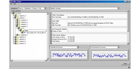
Result: The visualization panes on the right show information about the traffic on the selected flow.
-
Right-click on the selected flow in the treeview and choose Edit Attributes.
Result: The Attributes dialog box for this traffic flow opens.
The model (ip_traffic_flow) used to create this flow object has two attributes that specify the source-to-destination traffic:
- Traffic (bits/second)
- Traffic (packets/second)
These attributes describe the traffic data you just imported.

-
Click in the Value field of the Traffic (bits/second) attribute and choose Edit… from the pull-down menu.
Result: The Profile attribute dialog box opens.
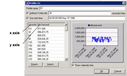
Each flow object contains one or more traffic profiles that specify the rate of traffic for that flow. A "profile" is an attribute that specifies data in an x-y format. In this case, the x scale specifies time intervals in seconds and the y scale specifies the traffic rate in bits/second over each interval.
-
Click OK to close the Profile dialog box, then OK to close the Attributes dialog box.
-
Click Close to close the Traffic Center.
Organizational Scaling
Now that you have a network loaded with traffic, you can begin to explore what will happen as the organization grows and traffic increases, first by 50 percent and then by 75 percent.
Riverbed Modeler can be used to model organizational scaling quickly and easily.
First, though, verify that your Network Simulation Repositories preference is set appropriately.
Procedure 4: Verifying the Repositories Preference
-
Choose Edit > Preferences.
-
Type network sim in the Search for: field and click the Find button.
-
If the Value field for the Network Simulation Repositories preference is not stdmod, click on that field.
Result: The Network Simulation Repositories dialog box opens.
-
Click the Insert button, then type stdmod in the field.
-
Click OK twice to close the Network Simulation Repositories and Preferences dialog boxes.
Now you can create a baseline.
Run the Simulation
Procedure 5: Running the Baseline Simulation
-
Choose DES > Configure/Run Discrete Event Simulation.
Result: The Configure/Run DES dialog box opens.
-
If the Simple… button appears in the lower-left corner, click it. This causes the Configure/Run DES dialog box to switch to the simple version.
-
Verify that the Duration is 1800 seconds.
-
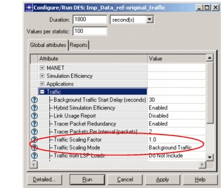
In the Global Attributes table, click the + next to Traffic to see the attributes in that group.
-
Verify that
- The Traffic Scaling Factor is 1.0
- The Traffic Scaling Mode is Background Traffic
(You might need to scroll down in the Global Attributes table to see these attributes.)
Figure 8: Configure Discrete Event Simulation Dialog Box
-
Click Run.
- 6.1 The simulation begins execution. When it is finished, click the Close button in the Simulation Execution dialog box.
You have generated a baseline for the results, but don't look at them just yet. Our interest is in seeing the effect of traffic growth, so we will look at these statistics when we can compare the results among all three scenarios.
Your task now is to create additional scenarios in which the background traffic is increased by 50 percent and 75 percent. The best way to do this is to duplicate the original scenario and then scale the traffic for each additional scenario.
For Traffic Increased by 50 Percent
Procedure 6: Running a Simulation with 50-Percent More Traffic
-
Choose Scenarios > Duplicate Scenario…
-
Name the new scenario scaled_50_percent.
-
In the new scenario, choose DES > Configure/Run Discrete Event Simulation.
-
If the Simple… button appears in the lower-left corner, click it. This causes the Configure/Run DES dialog box to switch to the simple version.
-
In the Global Attributes table, click the + next to Traffic to see the attributes in that group.
-
5.1 Change the Traffic Scaling Factor attribute to 1.5.
-
5.2 Verify that the Traffic Scaling Mode is set to Background Traffic (that is, flow traffic and baseline load traffic, but not explicitly generated traffic).
Figure 9: Traffic Scaling Factor is Set to 1.5

The next time you run a discrete event simulation, the background traffic in the network will be increased by 50 percent.
-
-
Click Apply to save your DES configuration and then click Cancel.
-
Save the project by choosing File > Save.
For Traffic Increased by 75 Percent
Procedure 7: Running a Simulation with 75-Percent More Traffic
-
Choose Scenarios > Switch To Scenario > original_traffic.
-
Duplicate the scenario and name the new scenario scaled_75_percent.
-
In the new scenario, choose DES > Configure/Run Discrete Event Simulation.
-
If the Simple… button appears in the lower-left corner, click it. This causes the Configure/Run DES dialog box to switch to the simple version.
-
In the Global Attributes table, click the + next to Traffic to see the attributes in that group.
-
5.1 Change the Traffic Scaling Factor simulation attribute to 1.75.
-
5.2 Verify that the Traffic Scaling Mode is set to Background Traffic.
The next time you run a discrete event simulation, the background traffic in the network will be increased by 75 percent.
-
5.3 Click Apply to save your DES configuration and then click Cancel.
-
5.4 Save the project by choosing File > Save.
You can run simulations for multiple scenarios with a single command from the Manage Scenarios... dialog box. You can also duplicate, delete, and rename scenarios.
Now that each scenario has been created with the appropriately scaled traffic, you can run the two new scenarios as a batch.
-
-
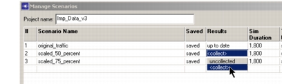
Choose Scenarios > Manage Scenarios…
Result: Notice that the Results for the original_traffic scenario are shown as up to date, while they are uncollected for the two new scenarios.
-
Change the Results fields for the scaled_50_percent and scaled_75_percent scenarios to
<collect>.Figure 10: Running Simulations from the Manage Scenarios Dialog Box
-
Click OK.
Result: The simulations begin execution. The two simulations should take about one minute to run. Close the DES Execution Manager dialog box when complete.
Now that all the results have been collected, you can view utilization on the links and FTP download response time to see how the network performs under various loads. To view utilization:
-
Right-click in the workspace and choose View Results from the pop-up menu.
-
Verify that the DES Graphs tab is selected.
-
Set the Results for: menu to Current Project.
-
In the top treeview, expand the
<initials>_Imp_Dataitem. Then make sure that all three scenarios for the project are selected. -
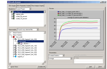
In the bottom treeview, expand Object Statistics > 192_9_200 > 192_9_200_Segment1_link_0[0] > point-to-point. Select utilization --->.
We want to compare the results, so display them all in one graph.
-
In the Presentation pane, change the top pull-down menu to Overlaid Statistics.
The utilization statistic will be more meaningful if viewed as the average utilization over time. You can apply a filter to the results to view the average utilization:
-
In the Presentation pane, change the bottom pull-down menu to average.
Figure 11: Presentation Options
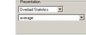
The following figure shows how the dialog box should be configured.
Figure 12: Utilization Preview in Results Browser
-
Click Show to display the graph.
Result: The utilization in each scenario for the 192_9_200_Segment1_link_0 object is graphed.
The graph for average utilization should be similar to the following figure.
Figure 13: Average Utilization Graph
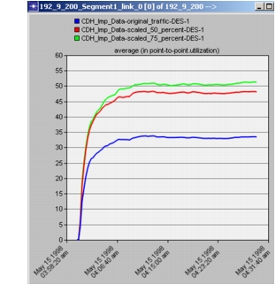
The low value of utilization (about 50 percent for the scaled_75_percent scenario) indicates that the between-LAN links are not the bottleneck in this network.
Also note that the x-axis is labeled with the actual times at which the data was collected. This information was contained as part of the imported traffic and was automatically set as the network start time.
The other statistic you collected was Download Response Time.
-
Move the Utilization graph out of the way, but don't close it.
-
In the bottom treeview, uncheck the checkbox for the utilization statistic.
-
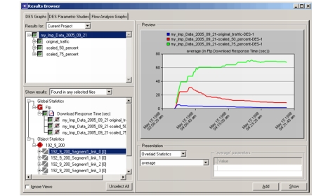
Expand Global Statistics > Ftp. Select Download Response Time (sec).
Figure 14: Download Response Time Preview in Results Browser
-
Click the Show button.
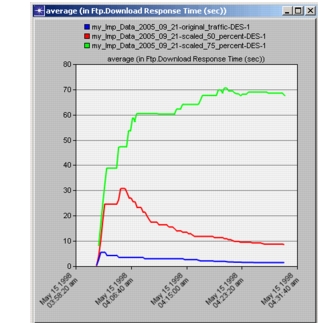
Figure 15: Average FTP Download Response Time Graph
-
Notice the following:
- When traffic is scaled 50 percent, the average download response time increases somewhat. (The initial "spike" is due to a large number of requests being made simultaneously. Because we ran the simulations for 30 minutes, we can see that this initial spike does not reflect the response times over a long duration.)
- When traffic is scaled up to 75 percent, the average response time increases even more. (The average download response time stabilizes at a considerably higher level due to traffic contention within the LANs.)
Although these increases are suggestive, you have run only one simulation set. For the results to be statistically useful, you might want to try different types of explicit traffic and vary the simulation seed.
You have now completed the Importing Traffic lesson.
- Select File > Save. We suggest saving the project so you can refer to it again if needed.
- Return to the Tutorials main menu and continue with the Expert Service Prediction (ESP) tutorial.
Note: Be sure to delete the stdmod setting for the Network Simulation Repositories preference when you are finished doing tutorials. To delete the setting, select Edit > Preferences, search for Network Simulation Repositories, click on the value, and choose Delete.