Small Internetworks
In this tutorial, you will see how Riverbed Modeler can do organizational scaling to solve a typical "what if" problem. You will learn how to use Riverbed Modeler features to build and analyze network models. This tutorial focuses on the use of the Project Editor and how it will be used with the Node and Process editors in later tutorials.
In this tutorial, you will
- Build a network quickly
- Collect statistics about network performance
- Analyze these statistics
Key Concept—In this tutorial, you will use the Project Editor to build a topology of a small internetwork, choose statistics to collect, run a simulation, and analyze the results.
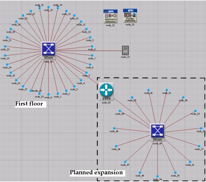
Suppose you are planning an expansion of a small company's intranet. The existing network is a star topology covering the first floor of the company's building. The expansion will add an additional star on another floor. You need to determine whether the existing network can handle the additional load. With Riverbed Modeler, you can build and test this "what-if" scenario.
Figure 1: The Final Network
Getting Started
You begin by creating a new project and scenario. A project is a collection of scenarios, and a scenario is a single network configuration that you can simulate and analyze.
After creating a new project, use the Startup Wizard to set up a new scenario. The options in the Wizard let you
- Define the initial topology of the network
- Define the scale and size of the network
- Select a background map for the network
- Associate an object palette with the scenario
Key Concept—The Startup Wizard automatically appears each time you create a new project. The Startup Wizard lets you define certain aspects of the network environment.
The following procedure describes how to use the Startup Wizard to set up a new scenario.
Procedure 1: Setting Up a New Scenario
-
If Riverbed Modeler is not already running, start it.
-
Select File > New…
-
Select Project from the pull-down menu and click OK.
-
Name the project and scenario, as follows:
-
4.1 Name the project
<initials>_Sm_IntInclude your initials in the project name to distinguish it from other versions of this project.
-
4.2 Name the scenario first_floor.
-
4.3 Click OK.
Result: The Startup Wizard opens.
-
-
Enter the values shown in the following table in the dialog boxes of the Startup Wizard.
Table 1: Values to Enter in the Startup Wizard
Dialog Box Name Value 1. Initial Topology Select the default value: Create empty scenario. 2. Choose Network Scale Select Office. Select the Use metric units checkbox. 3. Specify Size Select the default size: 100 m x 100 m 4. Select Technologies Include the Sm_Int_Model_List model family. 5. Review Check values, then click Finish. Result: A workspace of the size you specified is created. The object palette you specified opens in a separate window.
Creating the Network
Key Concept—Network models are created in the Project Editor using nodes and links from the object palette.
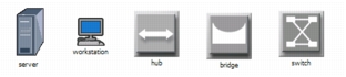
Node—A representation of a real-world network object that can transmit and receive information.
Figure 2: Nodes
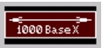
Link—A communication medium that connects nodes to one another. Links represent physical connectivity (e.g., electrical or fiber optic cables).
Figure 3: A Link
These objects are found in the object palette, a dialog box that contains graphical representations of node and link models.
If it is still open, close the object palette.
Key Concept—Use any of three methods to create a network topology, or a combination of all three. One method is to import the topology (discussed in a later tutorial). Another is to place individual nodes from the object palette into the workspace. The third method is to use Rapid Configuration.
Rapid Configuration creates a network in one action after you select a network configuration, the types of nodes within the network, and the types of links that connect the nodes.
Use the following procedure to o create the first-floor network with Rapid Configuration.
Procedure 2: Creating the First-floor Network with Rapid Configuration
-
Select Topology > Rapid Configuration…
-
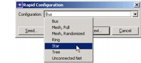
Select Star from the pull-down menu of available configurations, then click Next….
Figure 4: Available Configurations Pull-Down Menu
You will use this dialog box to specify the node models and link models in the network. Models follow this naming scheme:
Generic Devices:
<protocoln>_..._<protocoln>_<function>_<mod>Vendor Devices:
<Vendor>_<Chassis/Make>_<protocoln>where:
<protocoln>specifies a specific protocol supported by the model and the number of ports using that protocol<function>is an abbreviation of the general function of the model<mod>indicates the level of derivation of the model
For example:
ethernet2_bridge_int
specifies the intermediate (int) derivation of a 2-port Ethernet (ethernet2) bridge (bridge).
Vendor models have an additional prefix that specifies the vendor and the vendor product number for that particular network object.
For example, the 3Com switch used in this tutorial is named:
3C_SSII_1100_3300_4s_ae52_e48_ge3
This node is a stack of two 3Com SuperStack II 1100 and two Superstack II 3300 chassis (3C_SSII_1100_3300) with four slots (4s), 52 auto-sensing Ethernet ports (ae52), 48 Ethernet ports (e48), and 3 Gigabit Ethernet ports (ge3).
To specify the nodes and links to use to build the network:
Procedure 3: Specifying the Nodes and Links to Use to Build the Network
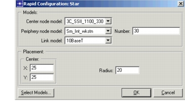
- Set the Center Node Model to 3C_SSII_1100_3300_4s_ae52_e48_ge3. This is a 3Com switch.
- Set the Periphery Node Model to Sm_Int_wkstn, and change the Number of periphery nodes to 30. This sets 30 Ethernet workstations as the peripheral nodes.
- Set the Link Model to 10BaseT.
Specify where the new network will be placed.
Procedure 4: Specifying Where the Network Will Be Placed
-
Set the X center and Y center to 25.
-
Set the Radius to 20.
Figure 5: Rapid Configuration Dialog Box
-
Click OK.
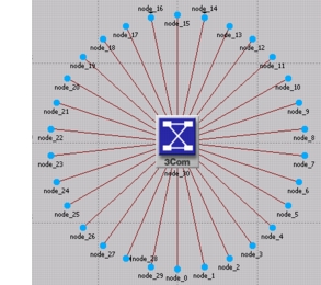
Result: The network is drawn in the Project Editor. To see it better, choose View > Zoom > To All.
Figure 6: The First Floor Network
Now that the general network topology has been built, you need to add a server. You will use the second method of creating network objects: dragging them from the object palette into the workspace.
Procedure 5: Creating Network Objects
-
Open the object palette by clicking on the Object Palette tool button.

-
Find the Sm_Int_server object in the palette and drag it into the workspace.
You will not find this exact server model on other object palettes because we created it with the correct configuration for this tutorial.
-
By default, you can create additional instances of the same object by left-clicking after the initial "drag-and-drop" from the palette.
Because you do not need additional copies of this model, right-click to turn off node creation.
Note: You also need to connect the server to the star network.
-
Find the 10BaseT link object in the palette and double-click on it.
-
Move the mouse from the object palette to the project workspace. Now click on the server object to draw one endpoint of your link, then click on the switch object in the center of the star to complete the link.
Result: A link is drawn, connecting the two objects.
-
Right-click to turn off link creation.
Finally, you need to add configuration objects to specify the application traffic that will exist on the network. Configuring the application definition and profile definition objects can be complicated, so you do not have to do these tasks right now. For this tutorial, we have included on the object palette:
- an application definition object with the default configurations of the standard applications, and
- a profile definition object with a profile that models light database access.
You need only drag the objects into your network. Doing so means that the traffic caused by workstations accessing a database at a low rate will be modeled.
-
Find the Sm_Application_Config object in the palette and drag it into the workspace
-
Right-click to turn off object creation.
-
Find the Sm_Profile_Config object in the palette, drag it into the workspace, and right-click.
-
Close the object palette.
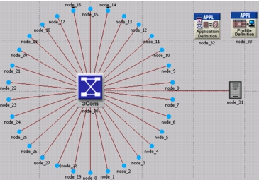
The network is now built and should look similar to the following figure.
Figure 7: The Finished First Floor Network
You are now ready to collect statistics.
First, however, let's explore the Node and Process Editors.
Key Concept—The Node and Process Editors are integral to the Riverbed Modeler workflow. The Node Editor is used to create node models that describe the internal flow of data within a network object. The Process Editor is used to create process models that describe the behavioral logic of a module in a node model.
Every node in a network has an underlying node model that specifies the internal flow of information in the object. Node models are made up of one or more modules connected by packet streams or statistic wires. Node modules in turn contain process models. A process model is represented by a state transition diagram (STD) that describes the behavior of a node module in terms of states and transitions.
Let's explore the node model that controls the server in the first floor network:
Procedure 6: Examing the Node Model
-
Double-click on node_31 (the Server object) in the Project Editor.
Result: The Node Editor opens as a new window within Riverbed Modeler.
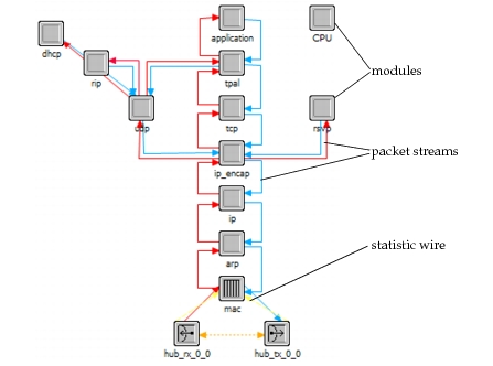
The following figure shows the node model within the Ethernet Server network object. The node model is made up of several different types of modules, which are described in the M/M/1 tutorial. Packet streams and statistic wires connect the modules.
Figure 8: Ethernet Server Node Model
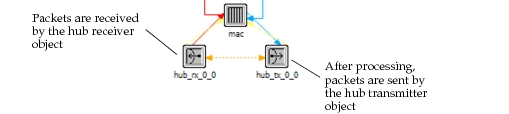
During a simulation, packets sent from a client machine are received by the hub receiver object (hub_rx_0_0) and processed up the protocol stack to the application module. After processing, they are sent down the stack to the transmitter (hub_tx_0_0), then back to the client machine.
Figure 9: Packet Processing by the Node Model
Next, let's look at the process model that defines the behavior of the tpal module. To view the process model:
-
Double-click on the tpal module in the Node Editor.
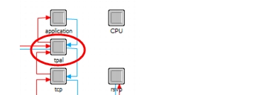
Result: The Process Model Editor opens in a new window.
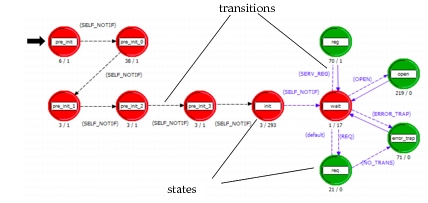
Figure 10: Example Process Model
-
Note the red and green states (these will be discussed in greater detail in the Basic Processes tutorial) and the solid and dotted lines indicating transitions between the states.
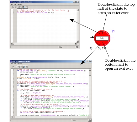
Each state in the process model contains an enter executive and an exit executive. Enter executives are executed when a process enters a state. Exit executives are executed when the process leaves the state. Operations performed in the state are described in C or C++.
-
Open an enter exec by double-clicking on the top half of the init state.
-
Open an exit exec by double-clicking on the bottom half of the state.
Figure 11: Opening the Enter Exec or Exit Exec of a State
-
Close both exec windows.
States are connected via transitions. Transitions can be either conditional (that is, they have a logical test that must be true before the transition occurs) or unconditional (no logical test).
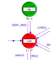
The following figure shows a conditional transition (the dotted line) from the wait state to the reg state. The condition SERV_REG must be true before the transition can occur. However, the transition from reg to wait (solid line) is unconditional, and occurs whenever the code in the reg state has finished execution.
Figure 12: Conditional and Unconditional Transitions
Later tutorials explore these editors in greater depth.
-
Close the Node and Process editors. If prompted, do not save changes.
Collecting Statistics
Key Concept—You can collect statistics from individual nodes in your network (object statistics) or from the entire network (global statistics).
Now that you have created the network, you should determine which statistics are needed to answer the questions presented earlier:
- Will the server be able to handle the additional load of the second network?
- Will the total delay across the network be acceptable once the second network is installed?
To answer these questions, you need a snapshot of the current performance for comparison. To get this baseline, you will collect one object statistic, Server Load, and one global statistic, Ethernet Delay.
Server load is a key statistic that reflects the performance of the entire network. To collect statistics related to the server's load, do the following procedure:
Procedure 7: Collecting Object Statistics
-
Right-click on the server node (node_31) and select Choose Individual DES Statistics from the server Object pop-up menu.
Result: The Choose Results dialog box for node_31 appears.
The Choose Results dialog box hierarchically organizes the statistics you may collect.
-
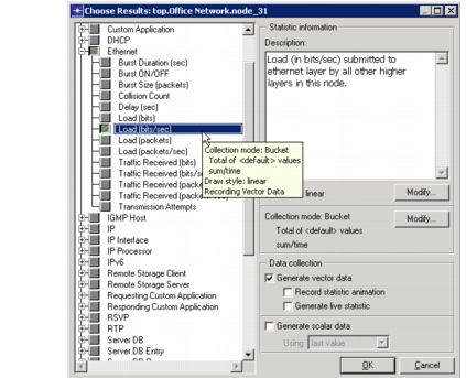
To collect the Ethernet load on the server:
-
2.1 Expand the treeview node for Ethernet in the Choose Results dialog box to see the Ethernet statistic hierarchy.
Note—The list of statistics can vary from the ones shown in this tutorial; they depend on the set of software components you have installed.
-
2.2 Click the checkbox next to Load (bits/sec) to enable collection for that statistic.
Figure 13: Choose Results Dialog Box
-
2.3 Click OK to close the dialog box.
-
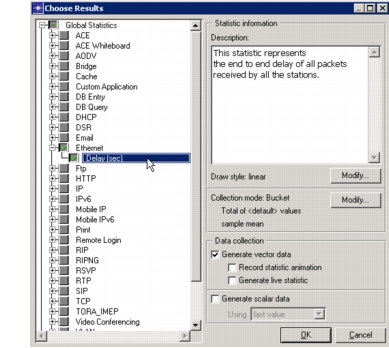
Global statistics can be used to gather information about the network as a whole. For example, you can find out the delay for the entire network by collecting the global Delay statistic:
Procedure 8: Collecting Global Statistics
-
Right-click in the workspace (but not on an object) and select Choose Individual DES Statistics from the workspace pop-up menu.
-
Expand the Global Statistics node.
-
Expand the Ethernet node.
-
Click the checkbox next to Delay (sec) to enable data collection.
Figure 14: Global Statistic Chosen
-
Click OK to close the Choose Results dialog box.
-
It is good to get into the habit of saving your project every so often. Choose File > Save, then click Save (the project already has a name, so you don't need to rename it).
Now that you have specified the statistics to collect and saved the project, you are almost ready to run your simulation.
First, though, verify that your Network Simulation Repositories preference is set appropriately.
Procedure 9: Verifying the Repositories Preference
-
Choose Edit > Preferences.
-
Type network sim in the Search for: field and click the Find button.
-
If the Value field for the Network Simulation Repositories preference is not stdmod, click on the field.
Result: The Network Simulation Repositories dialog box opens.
-
Click on the current value (such as "<empty>"), then click the Insert button.
-
Type stdmod and press Enter.
-
Click OK twice to close the Network Simulation Repositories and Preferences dialog boxes.
The following procedure describes how to run a simulation.
Procedure 10: Running a Simulation
-
Select DES > Configure/Run Discrete Event Simulation…
You can also open the Configure/Run DES dialog box by clicking on the Configure/Run Discrete Event Simulation (DES) tool button.

-
Click on the Detailed… button, if it is present.
-
Make the following changes in the dialog box:
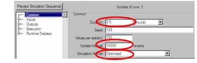
Figure 15: Configure Discrete Event Simulation Dialog Box
-
3.1 Type 0.5 in the Duration: field to simulate one-half hour of network activity.
-
3.2 Type 10000 (events) in the Update interval: field to specify how often the simulation calculates events/second data.
The simulation calculates and displays events/second data at 10,000-event intervals. The default setting for this is 500,000 for larger network simulations.
-
3.3 Set the Simulation Kernel to Optimized.
You can use one of two types of kernels to run your simulation. The development kernel collects simulation data you can use to debug your models, but the optimized kernel runs faster.
-
-
Click the Run button to begin the simulation.
While the simulation runs, a dialog box appears showing the simulation's progress.
Figure 16: Simulation Progress Dialog Box
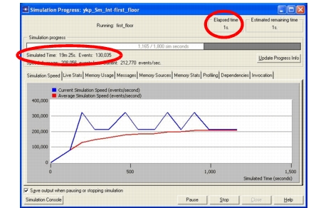
The dialog box above shows that, in 1 second of elapsed (actual) time, Riverbed Modeler has simulated 19 minutes and 25 seconds of network time. The entire simulation should take less than one minute to complete—the elapsed time varies according to the speed of your computer.
-
When the simulation finishes, the contents of the Messages tab appears. Click the Close button in the Simulation Sequence dialog box.
-
If your simulation does not complete, if no results were collected, or if the results vary significantly from those shown, you will have to troubleshoot your simulation. See "Troubleshooting Tutorials".
Viewing Results
After your simulation has executed, you will want to see the information collected for each statistic. There are several ways to view results; in this tutorial you will use the View Results option in the Workspace pop-up menu.
You will learn different ways to view results in later tutorials.
To view the server Ethernet load for the simulation:
Procedure 11: Viewing the Server Ethernet Load for the Simulation
-
Right-click on the server node (node_31) choose View Results from the server's Object pop-up menu.
Result: The Results Browser opens.
-
Expand the Object Statistics > Office Network > node_31 > Ethernet hierarchy.
-
Click on the checkbox next to Load (bits/sec) to indicate that you want to view that result.
-
Click the Show button in the Results Browser.
Result: The graph of the server load appears in the Project Editor, as shown in the following figure.
The graph of the server load should resemble the following graph. Your results may differ slightly due to differences in node placement and link length, but the general trends should be consistent.
Figure 17: Server Load Graph
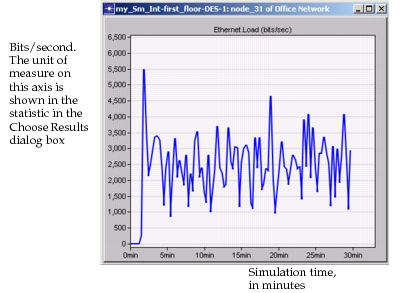
Note: At its peak, the load on the server is about 5,500 bits/second. You will need this baseline for comparison after you add the second network.
When you finish viewing the server load graph, close this dialog box and the Results Browser. (If the system prompts you, choose to delete the graph panel.)
Key Concept—The View Results option from the Workspace pop-up menu allows you to obtain global statistics and individual object statistics from one treeview.
You also should look at the Global Ethernet Delay on the network. To view this statistic:
Procedure 12: Viewing the Global Ethernet Delay Statistic
-
Right-click in the workspace, then select View Results from the pop-up menu.
-
Check the box next to Global Statistics > Ethernet > Delay (sec).
-
Click the Show button to view the Ethernet delay for the whole network.
Result: The Ethernet delay graph appears in the Project Editor. The graph should resemble the following figure.
Figure 18: Ethernet Delay Graph
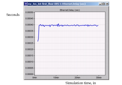
Note that after the network reaches steady state, the maximum delay is around 0.4 milliseconds.
When you finish viewing the graph, close the graph and the Results Browser.
Expanding the Network
You have created a baseline network and gathered statistics about it. Now you are ready to expand the network and verify that it still operates sufficiently well with the additional load.
When performing a "what-if" comparison, it is convenient to store the baseline network as one scenario and create the experimental network as a different scenario. You will duplicate the existing scenario and make changes to it instead of building the new topology from the beginning.
Procedure 13: Duplicating a Scenario
-
Choose Scenarios > Duplicate Scenario…
-
Enter expansion as the name for the new scenario.
-
Click OK.
Result: The scenario, with all the nodes, links, statistics, and the simulation configuration, is duplicated and named expansion.
The second-floor segment will resemble the first-floor segment, but will not have a server of its own.
Procedure 14: Building a New Segment
-
Select Topology > Rapid Configuration.
-
Choose Star for the topology and click Next…
-
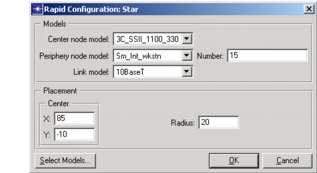
Complete the Rapid Configuration dialog box with these values:
- Center Node Model: 3C_SSII_1100_3300_4s_ae52_e48_ge3
- Periphery Node Model: Sm_Int_wkstn
- Number: 15
- Link model: 10BaseT
- X: 85, Y: -10, Radius: 20
Figure 19: Rapid Configuration Dialog Box
-
Click OK to create the network.
Next, join the two networks.
Procedure 15: Joining Two Networks
-
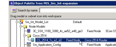
If it is not already open, click the tool button to open the object palette.

-
Expand the Cisco 2514 folder.
-
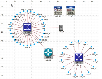
Drag the Cisco 2514 router icon into the workspace between the two networks. Right-click to turn off node creation.
-
Expand the Link Models folder and double-click on the 10BaseT link icon in the object palette.
-
Create 10BaseT links between the Cisco router (node_50) and the 3Com switches at the center of each star.
-
Right-click to turn off link creation.
-
Close the object palette.
-
Select File > Save.
The final network should resemble the following figure.
Figure 20: The Final Network
Next, run the expansion scenario.
Procedure 16: Running the Expansion Scenario
-
Select DES > Configure/Run Discrete Event Simulation…
-
Click the Detailed… button, if it appears, and verify that the Duration is set to 0.5 hours and the Update interval is set to 10000.
-
Click the Run button to begin the simulation.
Figure 21: Simulation Progress Dialog Box, Simulation Speed Tab Selected
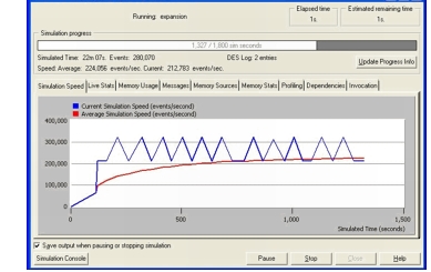
Result: As before, a window displays simulation start-up messages first, and then an animated graph shows both the current and average speed in events per second during the simulation. When the simulation is completed, you can view the event/second graph results from the Simulation Speed tab.
-
When the simulation is done, close the Simulation Progress dialog box. If you had problems, see "Troubleshooting Tutorials".
Comparing Results
To answer the questions posed about the addition of a second network to the existing LAN, you need to compare the results from both of the simulations you ran.
You will use the View Results menu item in the Object and Workspace pop-up menus to combine statistics from different scenarios in the same graph. When comparing results, choosing a statistic in one scenario produces a graph showing the value of that statistic in all scenarios.
To view the server load from both scenarios at once:
Procedure 17: Viewing the Server Load from Both Scenarios
-
Right-click on the server node (node_31) to display the pop-up menu and choose View Results.
-
Select Current Project from the Results for: pull-down menu.
-
Select the box next to each of the two scenarios.
-
In the Presentation area, select Overlaid Statistics from the pull-down menu.
Note: If your results differ radically from those shown in the following figures, you will have to troubleshoot your simulation. See "Troubleshooting Tutorials".
-
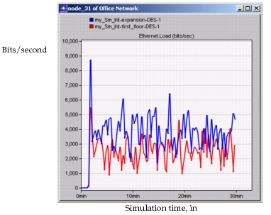
Select the Object Statistics > Office Network > node_31 > Ethernet > Load (bits/sec) statistic and click the Show button. Your results should resemble those in the following figure (but may not be identical):
Figure 22: Ethernet Loads Compared
The following graph is the time average of the Ethernet load between the baseline (first_floor) scenario and the expansion scenario. You will learn how to create a graph of the time average in the next tutorial.
Figure 23: Time-Averaged Server Load Compared
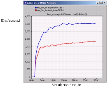
Note: Although the average load for the expansion scenario is higher (as expected), the load as a whole appears to be leveling off (that is, not monotonically increasing), indicating a stable network.
Next, see how much the network's delay is affected by adding a second floor. To compare Ethernet delay for the two scenarios:
-
Close the graph and the Results Browser for the server.
-
Right-click in the workspace to display the pop-up menu and choose View Results.
-
As before, select Current Project from the Results for: pull-down menu, then select the box next to each of the two scenarios.
-
Under Show Results, select Global Statistics -> Ethernet -> Delay (sec).
-
In the Presentation area, select Overlaid Statistics from the pull down menu.
-
Click the Show button to display the graph.
-
Your graph of Ethernet Delay should resemble the following figure.
Figure 24: Ethernet Delay Compared
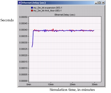
This graph shows that there is no significant change in Ethernet delay on the network. Although server load has increased, delay has not.
-
Close the graph and the Results Browser.
-
Select File > Close and save changes before closing.
Now you are ready to go on to the M/M/1 Queue tutorial. This tutorial explores the use of node models in the workflow. Return to the main tutorial menu and choose M/M/1 Queue from the list of available tutorials. Or, if you prefer, choose another tutorial of interest.
Note—Be sure to delete the stdmod setting for the Network Simulation Repositories preference when you are finished doing tutorials. To delete the setting, select Edit > Preferences, search for Network Simulation Repositories, click on the value, and choose Delete.