Predicting Application Deployment with Transaction Analyzer Models
Transaction Analyzer includes predictive features that enable you to determine how network and application changes will affect application performance. This tutorial demonstrates how you can import traffic from Transaction Analyzer to create a “virtual deployment” to test a proposed application’s performance. You will build a model and predict the performance of an application deployment to a large group of users.
“Workflow: Running a Discrete Event Simulation”.The starting point is a series of transactions for a three-tier Oracle application; these transactions have been captured in a test lab using a local area network (LAN) environment. The requirement is to predict bandwidth needs and performance when this application is deployed on a wide area network (WAN).
The goal of this exercise is to answer the following questions:
- What is the response time for a single user on the 256 Kbps Frame Relay circuit?
- Can a 256 Kbps Frame Relay circuit support 200 users?
- How much bandwidth will 200 users need?
- With the existing traffic load on the circuit, will performance for 200 users be satisfactory?
The original packet traces were captured in a test lab where the application was deployed to a sample client machine on the same LAN as the Application and Database (DB) Servers.
Figure 1: Test Lab Topology
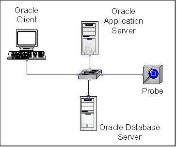
Transaction Analyzer used the packet traces to create application fingerprints that characterize the data exchange between tiers. From these fingerprints, a simulation can show how the application will behave under different conditions.
Six separate transactions (Connect, Login, List Categories, Choose Category, View Record, and Logout) are used to build the application definition.
The Data Exchange Chart for each transaction is shown in the following figures.
Figure 2: Step 1: Connect
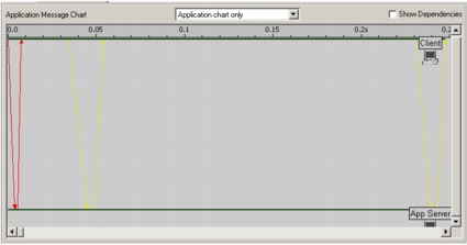
Figure 3: Step 2: Login
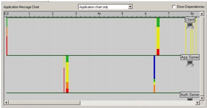
Figure 4: Step 3: List Categories
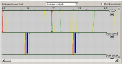
Figure 5: Step 4: Choose Category
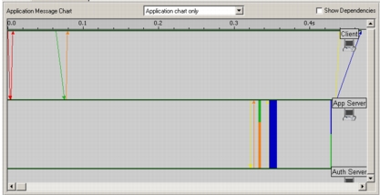
Figure 6: Step 5: View Record
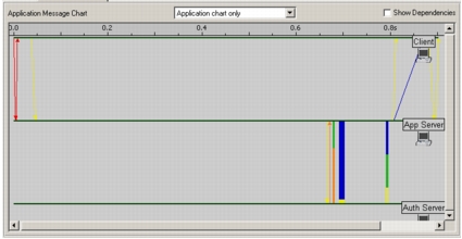
Figure 7: Step 6: Logout
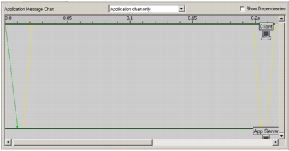
Import the Transaction Analyzer Model
Note: If you have a Transaction Analyzer Plus license and want to run a discrete event simulation (DES), download and run IT Guru 16.0 or later. IT Guru will allow you to run DES using the Transaction Analyzer Plus license.
For more information, see “Workflow: Running a Discrete Event Simulation”.
The topology wizard builds network models from Transaction Analyzer models and defines settings that are specified during the import.
Procedure 1: Import the Transaction Analyzer Model into Riverbed Analysis Software
-
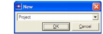
Open your Riverbed analysis software (such as SteelCentral NetPlanner or Riverbed Modeler), choose File > New…, select Project from the pull-down menu, and click OK.
-
Enter <initials>_App_Deploy as the project name. Name the scenario single_user.
Verify that the Use Startup Wizard when creating new scenario checkbox is selected. If not selected, click the checkbox to select it.
Click OK.
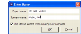
Result: The Startup Wizard appears.
-
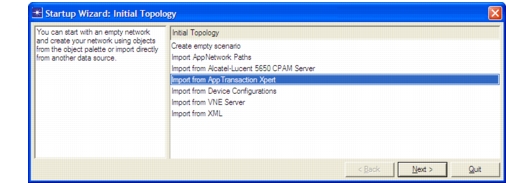
In the “Startup Wizard: Initial Topology” dialog box, notice that you can import topologies from a variety of sources, including device configurations and XML files.
-
Select Import from Transaction Analyzer. Click Next >.
Configure the Application
Perform the following procedure to configure the application.
Procedure 2: Configuring the Transaction Analyzer Application
-
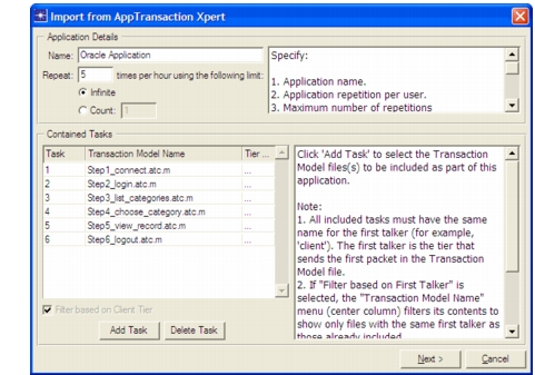
Set the Name field to Oracle Application. This text string identifies the application in the model.
-
Set the Repeat field to 5. This field controls how many times a user executes the application per hour.
-
Leave the limit at the default value, Infinite.
-
Click on Add Task. In the Contained Tasks table, click on the word Specify…, and then select Step1_connect.atc.m from the pull-down menu.
-
Repeat the previous step five more times to add the following tasks to the Contained Tasks list:
- Step2_login.atc.m
- Step3_list_categories.atc.m
- Step4_choose_category.atc.m
- Step5_view_record.atc.m
- Step6_logout.atc.m
The dialog box should look like the one shown in the following figure.
Figure 8: Import from Transaction Analyzer Application Dialog Box
-
Click Next >.
Create the Topology
Perform the following procedure to create the topology for one user of the application on a 256 Kbps Frame Relay circuit with 40 ms of latency.
Procedure 3: Create the Topology
-
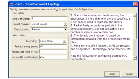
In the LAN Details section of the dialog box, verify the following settings:
- Number of Clients: 1
- Packet Analyzer: Do Not Include
- Client Location: Remote
-
In the WAN Details section of the dialog box, specify the following settings:
- Technology: Frame Relay
- Packet Latency: 40
- Packet Loss Ratio: 1
- Access Bandwidth: 256
The dialog box should look like the one shown in the following figure.
Figure 9: Create Transaction Analyzer Topology Dialog Box
-
Click Create.
Review the Model
The Wizard creates a topology similar to the one shown in the figure below. The Tasks, Applications, and Profiles objects have been configured according to the packet traces and the entries that you made in the Wizard. You can customize them further, if necessary.
Figure 10: Topology for One User Over 256 Kbps Frame Relay PVC
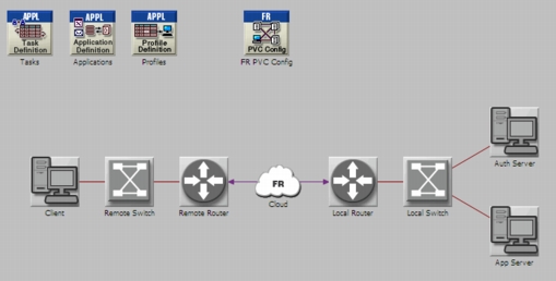
The topology consists of the Client, the Oracle App Server, and the Oracle Auth Server, which are assigned traffic profiles based on the imported Transaction Analyzer models. Access links connect switches and routers through a Frame Relay cloud.
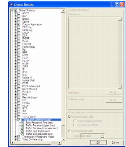
The Wizard selects statistics that are commonly used in application deployment studies. You can select additional statistics or deselect statistics that are already selected.
Procedure 4: Selecting and Deselecting Statistics
-
To inspect the statistics that have been selected, choose DES > Choose Individual Statistics…
Figure 11: Statistics to be Collected by the Simulation
-
Examine the statistics that are available and the statistics that have been selected. Click Cancel when done.
-
Select File > Save, and then click Save to save the project.
Run the Simulation
Now that the topology is created, you can run the simulation. The application will be activated five times per hour on a 256 Kbps Frame Relay circuit with 40 ms of latency.
Procedure 5: Running the Simulation
-
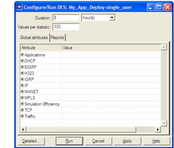
Click the Configure/Run Discrete Event Simulation toolbar button.
Result: The Configure Discrete Event Simulation dialog box appears. If the dialog box is in the Detailed view, click the Simple button in the lower-left corner.
Figure 12: Configure Discrete Event Simulation Dialog Box
-
Set the Duration value to 8 hours. Keep the default values for all other fields, and then click Run.
-
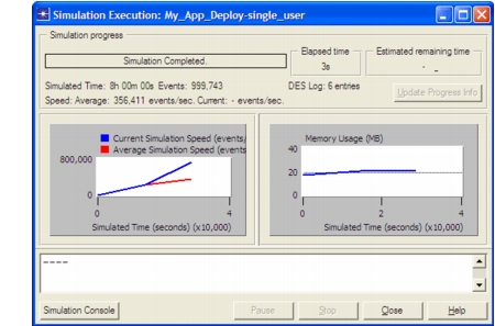
Notice that the Simulation Execution dialog box provides a running update of the simulation as it progresses.
Figure 13: Simulation Execution Dialog Box
-
Close this dialog box when the simulation completes.
View Results
Now view the response time for the individual tasks and the entire application.
Procedure 6: Viewing the Results
-
Click the View Results toolbar button.
Result: The Results Browser displays. The Show results panel in the lower-left corner provides a treeview for available statistics.
-
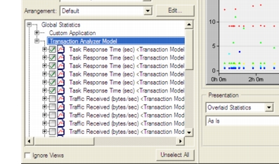
Expand the Global Statistics > Transaction Analyzer Model hierarchy by clicking on the + sign (arrow on Linux platforms) in the “Show results” pane. Scroll down and select the six Task Response Time statistics.
-
Set the view (pull-down menu under Presentation) for Overlaid Statistics.
Figure 14: Select Statistics to View in a Graph
-
Click Show.
Note: Your results may be slightly different because the repetition rate is based on a random (exponential) distribution.
Figure 15: Response Time Statistics for the Individual Tasks
-
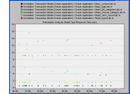
You see the response times of the individual tasks vary from about 0.5 seconds (Step1_connect) to over 10 seconds (Step2_login). You may see a different number of data points or a different start time. This occurs because the start time and repeatability are determined by exponential distributions.
-
In the Results Browser dialog box, click Unselect All.
Now view the response time for the entire application.
-
Collapse the Global Statistics > Transaction Analyzer Model hierarchy by clicking on the – sign (< on Linux).
-
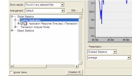
Expand the Custom Application hierarchy by clicking on the + sign, and then select the Application Response Time (sec) statistic.
-
Change the filter menu from As Is to average.
Figure 16: Select the Application Response Time Statistic
-
Click Show.
Figure 17: Average Response Time for Entire Application
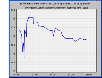
Result: The graph shows that the entire application had a response time of over 15 seconds. The application response time is the time it takes to complete all the tasks of the application.
You may see a shorter or longer curve (because the number of times the application repeats is based on a probability distribution) or a different start time.
Note: The outlier point that raises the average occurs because this model drops 1 percent of the packets on the Frame Relay cloud. Dropped packets cause TCP to retransmit; these retransmissions increase the average response time.
Now you can answer the first question posed in the Overview: the response time for a single user on the 256 Kbps circuit is over 16 seconds.
-
Close the graph panels and the Results Browser dialog box.
-
When prompted, click Hide.
This enables you to view the results later by clicking on the Hide/Show Graph Panels button.
-
Select File > Save to save the project.
Simulate Multiple Users
Now that you know the response time for a single user, you want to see the response time for many simultaneous users over a Frame Relay circuit. You will create a new scenario that demonstrates the behavior of the application when deployed to 200 users.
Procedure 7: Simulating Multiple Users
-
Select Scenario > Duplicate Scenario…
-
Name the scenario 200_Users, and then click OK.
-
Right-click on the client and choose Edit Attributes (Advanced).
-
Change the model attribute from ethernet_ace_wkstn to 100BaseT_LAN.
- 4.1 Click on the Model attribute value.
- 4.2 If a warning dialog box displays, select Yes.
- 4.3 From the pull-down list, select 100BaseT_LAN.
-
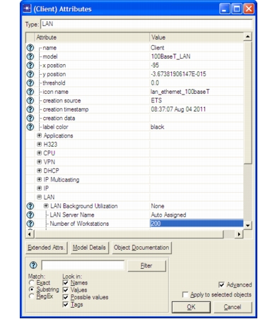
Expand the LAN attribute: click on the + sign (arrow on Linux platforms). Change Number of Workstations from 10 to 200. Click OK to close the window.
-
Click on the Configure/Run Discrete Event Simulation button. In the Configure/Run DES dialog box, change the Duration to 0.5 (hours). Click Run. This simulation may take a few minutes to complete.
-
Close the dialog box when the simulation completes.
View Results for Multiple Users
Now you can look at the application behavior for 200 users.
First, look at the global statistics for the tasks and application.
Procedure 8: Viewing Results for Multiple Users
-
Click the View Results toolbar button.
-
Expand the Global Statistics > Transaction Analyzer Model hierarchy. Scroll down and select the six Task Response Time statistics.
-
Set the view (left pull-down menu) for Overlaid Statistics.
-
Click Show.
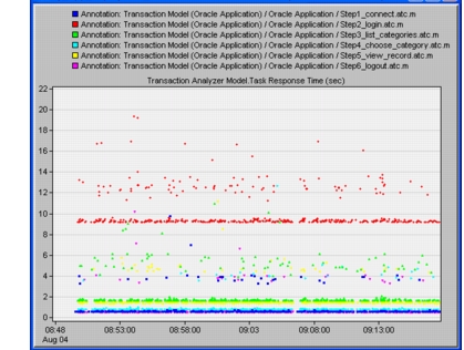
Note: The colors assigned to the statistics in the graph are determined by the order in which the statistics were selected in step 2; therefore, the colors in your graph may differ from the colors in the examples.
Figure 18: Response Time Statistics for the Individual Tasks for 200 Users
-
In the View Results dialog box, click Unselect All.
-
Collapse the Transaction Analyzer Model hierarchy by clicking on the – sign.
-
Expand the Custom Application hierarchy, then select the Application Response Time (sec) statistic.
-
Click Show.
Figure 19: Response Time for Entire Application for 200 Users
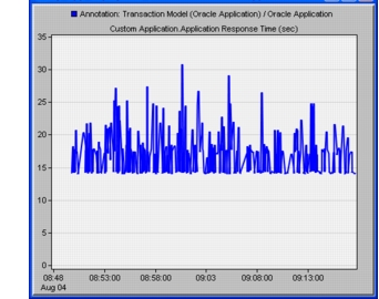
Your graph might vary slightly from the figure above, but the trend should be similar.
The graph shows an average response time of over 15 seconds for 200 users; this is in the same range as the delay experienced by one user. You can verify the average by using the average filter.
-
Save the project and close the Results Browser dialog box.
-
Click on the Hide/Show Graph Panels button to hide the current results.
This answers the second question posed in the Overview: the 256 Kbps Frame Relay link can support the 200 users in the remote site.
Now, look at the throughput for a specific link.
-
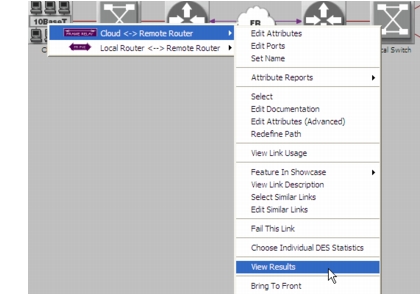
Right-click on the link between the Cloud and the Remote Router, and then select View Results from the pop-up menu. (If a menu with multiple items displays, choose Cloud <-> Remote Router, and then select View Results from the pop-up menu.)
Figure 20: Select the Remote 256 Kbps Link
-
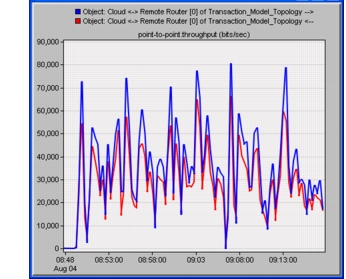
Expand the Object Statistics hierarchy until point-to-point is expanded. Then select the two statistics for throughput (bits/sec) and choose Overlaid Statistics.
-
Click Show.
Figure 21: Throughput on the WAN Link for 200 Users
-
This graph shows instantaneous throughput. To see this data as an average, apply the moving average filter.
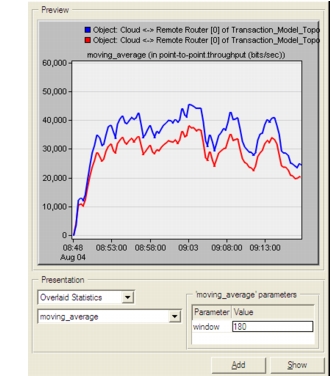
In the Results Browser dialog box, change the filter from As Is to moving_average.
Figure 22: Apply the moving_average Filter to the Throughput Statistic
-
In the moving_average parameters box, enter a window value of 180 seconds.
-
Click Show.
-
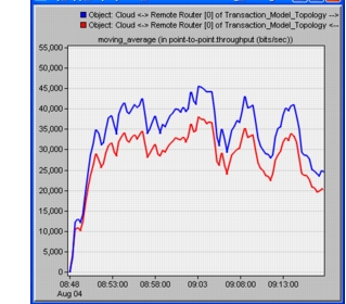
Review the throughput displayed as a moving average. Your results may vary slightly.
The moving average filter groups data into “buckets” of a specified size (180 seconds in this example), calculates the average of all data points in the bucket, and then creates a graph from the average for each bucket. This filter removes the extremes but shows how throughput changes over time.
Figure 23: Throughput with moving_average Filter
-
Save the project and close the Results Browser dialog box.
-
Click on the Hide/Show Graph Panels button to hide the current results.
This answers the third question posed in the Overview: 200 users consume an average of 30 Kbps of the available 256 Kbps.
However, this simulation is a simplified and optimistic analysis. In reality, the WAN circuit is already carrying traffic from other applications, and during a typical business day, the 256 Kbps WAN link is 80 percent utilized. Your analysis of this application rollout should incorporate the existing traffic.
Simulate Multiple Users with Existing Traffic
The simplest way to simulate the existing traffic is to apply background utilization traffic to the WAN.
The simulation run in this section can take up to 10 minutes to complete, depending on the speed of your computer.
Procedure 9: Simulating Multiple Users with Existing Traffic
-
Select Scenario > Duplicate Scenario… Name the new scenario 200_Users_w_background_load, and then click OK.
-
Set a bidirectional background load of 200 Kbps on the Cloud <-> Remote Router link:
-
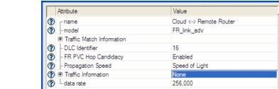
2.1 Right-click on the link between the Remote Router and Cloud, and select Edit Attributes from the pop-up menu. (If a menu with multiple items appears, choose Cloud <-> Remote Router, and then select Edit Attributes from the pop-up menu.)
Figure 24: Edit Attributes Dialog Box—Detail
-
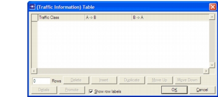
2.2 Change the Value field of Traffic Information from None to Edit…
-
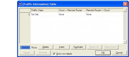
2.3 Change the value of the Rows field to 1 and press Enter.
-
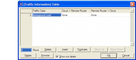
2.4 Change the value of Traffic Class to Background Load and press Enter.
-
2.5 Click on the cell under Cloud -> Remote Router and select Edit.
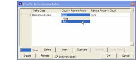
Result: The (A -> B) attribute table appears. The table contains attributes for specifying unidirectional traffic on the link.
-
2.6 Change the Value field of Traffic Load (bps) from NONE to Edit…
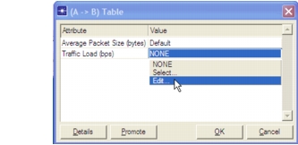
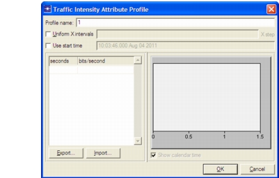
Result: The Traffic Intensity Attribute Profile window appears. You can use this window to define, view, and edit background load traffic from the Cloud to the Remote Router.
-
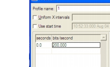
2.7 Enter 0.0 seconds and 200,000 bits/second as shown in the following figure:
-
2.8 Click OK to save this background load, which is about 80 percent of the 256 Kbps link speed.
Result: This specifies the background load of 200 Kbps background load from the Cloud to the Remote Router.
-
2.9 Specify the same 200 Kbps load in the opposite direction (that is, from the Remote Router to the Cloud): Repeat Steps 2.5 through 2.8 for the background load in the Remote Router -> Cloud direction.
-
2.10 Click OK to close the (Traffic Information) Table.
-
2.11 Click OK to close the Cloud <-> Remote Router Attributes window.
-
-
Click the Configure/Run Simulation toolbar button. In the Configure Discrete Event Simulation dialog box, leave the duration as 0.5 hour. Click Run.
-
Close this dialog box after the simulation finishes.
These results show how the link utilization impacts the application response time.
-
Click the View Results toolbar button.
-
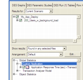
Expand the Custom Application hierarchy. Select Application Response Time (sec).
Figure 25: Select the Application Response Time (sec) Statistic
-
Click Show.
Figure 26: Response Time for 200 Users on 80% Utilized WAN Link
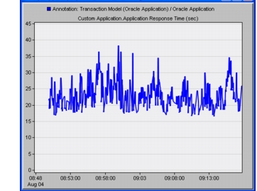
You might see higher or lower spikes, but most response times should be 20–25 seconds.
-
Notice that at certain times, the response time spikes up much higher. What is the link utilization during those periods?
-
Close the Results Browser dialog box.
-
Right-click on the link between the Remote Router and the Cloud, and then choose View Results.
-
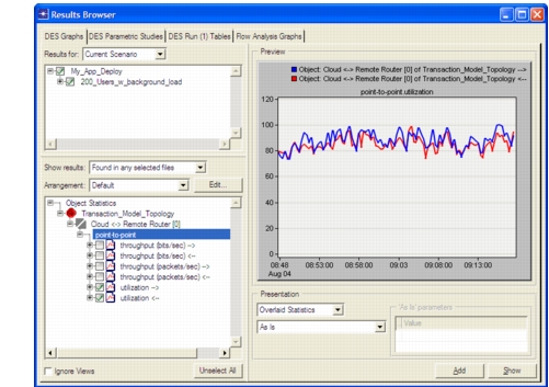
Select both utilization statistics, specify Overlaid Statistics, and then set the filter to As Is.
Figure 27: Select the Utilization Statistics
-
Click Show.
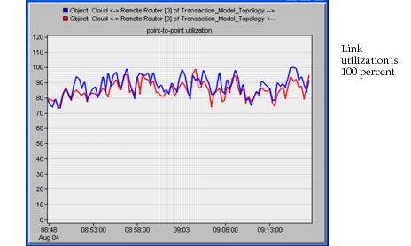
Figure 28: Utilization on 256 Kbps Frame Relay Circuit
-
Click the Hide/Show Graph Panel button to hide the displayed results.
-
Save and close the project.
Now you can answer the final question: this scenario shows that there will be significant performance problems if this application is deployed to the 200 remote users. When you model the existing 80 percent load, response times will vary from over 15 seconds, as predicted by the second scenario, to much higher spikes.
The utilization graph shows that these spikes in application response time correspond to periods of link congestion. There are several instances where the WAN link reaches 100 percent utilization.
This scenario suggests that the 256 Kbps WAN link should be upgraded before deploying this application.