Server Configuration Object Attributes
The Server Configuration object has several attributes describing the underlying server hardware. Hardware attributes described in the Server Configuration object are listed below:
Figure 482: Server Configuration Object Attributes
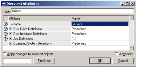
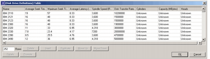
- Disk Drive Definitions. This attribute specifies hardware characteristics of common disk drives. Default values are obtained from manufacturer data sheets.
Figure 483: Disk Drive Definitions Attribute
-
Name. This attribute describes the physical drive; it usually includes the manufacturer name and model number.
-
Average Seek Time. This attribute specifies the average time required for the drive’s read/write head to position itself over the correct track.
-
Maximum Seek Time. This attribute specifies the time required for the read/write head to travel from the first track to the last, or vice versa. It is similar to the Average Seek Time but limited by the drive’s physical geometry.
-
Average Latency. This attribute specifies the amount of time required for the drive to rotate to the correct position for the read/write operation to occur.
-
Spindle Speed. This attribute specifies the maximum latency, which is determined from the rotational speed of the drive. The time required for one disk revolution is the maximum latency a drive can produce.
-
Disk Transfer Rate. This attribute specifies the maximum rate at which data can be transferred over the drive’s interface bus (a drive may have faster internal transfer rates, however).
-
Cylinders. Number of physical cylinders on the disk drive. This attribute value is not used by the server disk model.
-
Capacity. The storage capacity of the disk drive in Megabytes. This attribute value is not used by the server disk model.
-
Heads. Number of physical heads in the disk drive. This attribute value is not used by the server disk model.
-
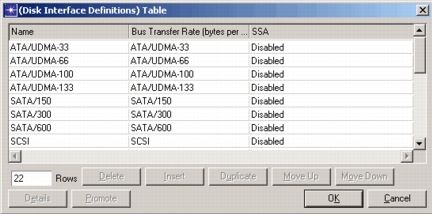
Disk Interface Definitions. The interface is a shared bus device that controls a variable number of disk drives. Many standard configurations are presented with the following attributes:
Figure 484: Disk Interface Definitions Attribute
-
Name. This attribute specifies a user-defined value that describes the physical interface. This typically includes the interface standard and any RAID (Redundant Array of Inexpensive Disks) configuration used by the device.
-
Bus Transfer Rate. This attribute specifies the maximum data transfer rate between the drives and the interface. The actual transfer rate may be lower if the drives are slower. Only one drive can transfer data at a time.
-
SSA - Serial Server Architecture. This is a standard developed by IBM to increase interface throughput by providing two read and two write buses. This allows up to four data transfer operations to occur concurrently, as long as they are to separate physical drives.
-
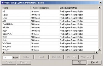
Operating System Definitions. This attribute specifies operating system descriptions that include information on the default operating system and scheduling method used by the operating system.
Figure 485: Operating System Definitions
-
Name. A user-defined value which uniquely describes the operating system definition.
-
Timeslice. This is the maximum amount of time a job will use the processor before giving up the CPU to another process. In general, smaller time slices will produce more events, resulting in longer simulation times.
-
Scheduling Method. The algorithm used to dispatch jobs to processors. Currently two scheduling methods have been defined:
-
Round-Robin. The algorithm schedules the first available highest priority job at the start of a timeslice or when the processor becomes free. The algorithm does not allow jobs to be pre-empted when a higher priority job becomes available.
-
Pre-Emptive Round-Robin. The algorithm schedules the first available highest priority job at the start of a timeslice or when the processor becomes free. If a job becomes available when all the processors are busy, the lowest priority job with priority less than the newly available job, is preempted, so that the new job may execute.
-
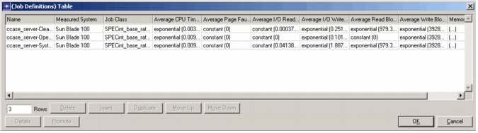
Job Definitions. This attribute specifies workload descriptions that include information on the measured performance of server jobs. These job definitions are independent of the servers they run on. When multiple copies of a job exist, the information is distilled into a single representative ‘instance’ that can then be scaled. The attributes described here apply to the representative instance:
Figure 486: Job Definitions Table
-
Name. A user-defined value which uniquely describes the workload. Note: Job name remote_access is reserved and cannot be specified in the job definitions table. see the discussion of Job Definitions attribute in the Server Attributes section.
-
Measured System. When simulating jobs for systems other than the one on which the measured values were obtained, the model needs to know how to scale these values. This attribute, along with the job class, allows scaling to be performed. The server description for this system must already exist before this value can be obtained.
-
Job Class. As different jobs have different performance characteristics, each job can be assigned it’s own ‘class’. This value is obtained from the list of job classes provided for the server described in the ‘Measured System’. Since this value is used to scale jobs, it must exist in both the measured system described above, and in the target system described on the individual server.
-
Average CPU Time. A distribution describing the amount of processor time consumed by the job.
-
Average Page Faults. A distribution describing the number of page faults generated by a single job instance. This includes both hard (those requiring an I/O operation to exchange data with that on disk) and soft faults (those with data found in memory).
-
Average I/O Reads/Writes. Distributions describing the typical I/O behavior of the job. These I/Os will be distributed evenly over the life of the job.
-
Average I/O Read/Write Blocksize. Distributions describing the amount of data transferred by a single I/O operation. This will affect the I/O processing time.
-
Memory Requirements. Memory usage is also tracked on a single instance basis. Since many applications use a minimum amount of memory regardless of the number of active instances, it may be desirable to define a job that consumes no resources other than memory to represent this baseline requirement.
Figure 487: Memory Requirements Table
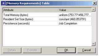
- Total Memory. All memory used by a job, including that resident in memory (the Resident Set Size), and that which is contained in swap.
- Resident Set Size. The amount of physical memory consumed by a job. This does not include any memory that resides in swap.
- Persistence. A distribution describing how long the memory is required. Typically this is set to Job Completion, which means the memory is relinquished when the job finishes. If the memory remains in use throughout the simulation, this should be set to ‘End of Simulation’.
Server Definitions Editor
The Server Library provides the interface to the server definitions stored in an external file. The same dialog box is displayed from both the Server Characterization Editor (SCE) and the project editor.
The Server Definition dialog box allows you to view and edit current server definitions, and create new server definitions. From the Project Editor, the server definitions can be accessed from the menu Protocols > Servers > Open Server Library (or in the SCE main window from the Hardware > Server Definitions... menu item). The following figures illustrate how this editor works.
Figure 488: Server Library Dialog Box
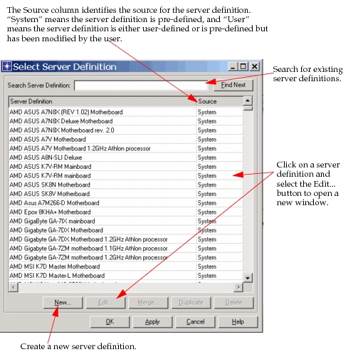
Figure 489: Duplicate Server Definition
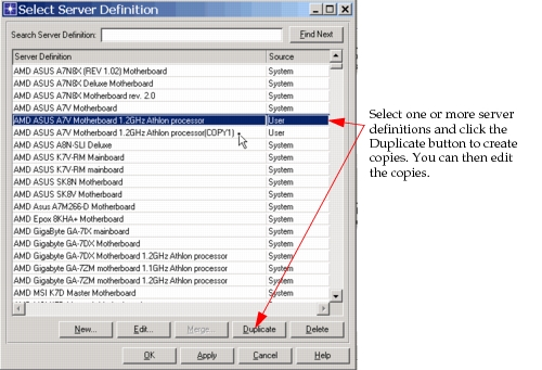
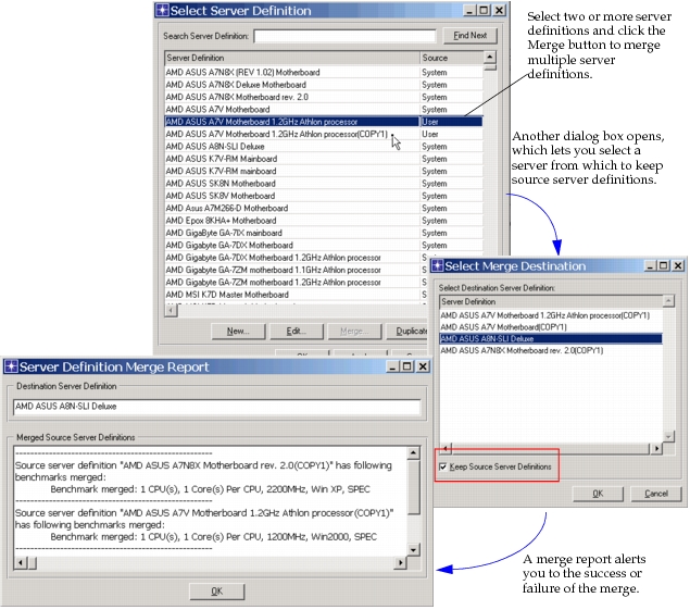
Figure 490: Merge Server Definitions
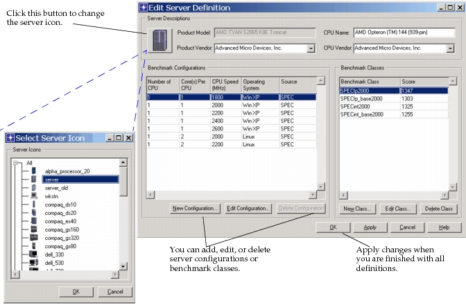
When you choose to edit a server definition, the dialog box shown in the following figure appears. Editable fields are described in the next section.
Figure 491: Edit Server Definition Dialog Box
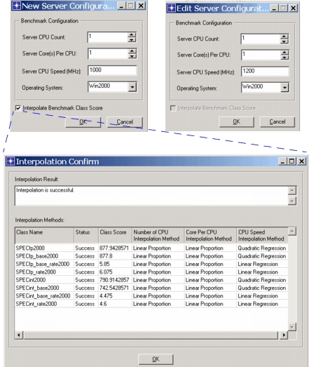
If you select the New Configuration... or Edit Configuration... button, a new dialog box appears, shown in the following figure. You can edit the number of CPUs, the number of cores per CPU, CPU speed, and the operating system. When you create a new server configuration, you can also choose to interpolate the benchmark class scores based on known data points.
Figure 492: New/Edit Configuration Dialog Box
- Product Model. A pre-defined value that describes the server. It typically includes the manufacturer’s name and model number. This value is combined with specific server configuration information to generate a unique key. That key is further referenced by job definitions to identify the system on which the job was measured.
- Product Vendor. This attribute specifies the manufacturer of the server. This attribute is not used by the server models, it is intended to be used by SCE for server matching.
- CPU Model. A user-defined value that describes the server. It typically includes the manufacturer’s name and model number.
- CPU Vendor. This attribute specifies the manufacturer of the processors used in the server. This attribute is not used by the server models, it is intended to be used by SCE for server matching.
- Number of CPUs. This attribute specifies the number of actual microprocessors contained in the system. Every microprocessor may contain one or more “cores”. This attribute is used by Server Characterization Editor (SCE) for new benchmark class score interpolation.
- Core(s) Per CPU. This attribute specifies the number of microprocessor cores contained in the CPU. Every core is an architectural, computational processing element. This attribute is used by SCE for new benchmark class score interpolation.
- CPU Speed (MHz). This attribute specifies the speed (in MHz) of processors used in the server. The value is used by SCE for new benchmark class score interpolation.
- Operating System. This attribute specifies the operating system on which the benchmark programs were executed. The operating system value refers to an entry in the Server Config object’s Operating System Definitions attribute: which identifies the timeslice and scheduling algorithm to be used.
- Source. This attribute identifies the source of the server configuration. “SPEC” means that this server configuration and its corresponding benchmark class information are directly from SPEC web site. “User” means this server configuration is either defined by the user or is pre-defined but has been modified by a user.
- Benchmark Classes. This is a list of standard benchmark classes and scores supported by the server. The predefined server configurations include the CPU2000 and CPU95 benchmarks published at http://www.spec.org. For multi-processor systems, the rate values have been divided by the number of processors to provide a ‘per-processor’ rating.
Interpolation Methods
The server model supports benchmark class score interpolation, that is, a newly-created server configuration can automatically generate its benchmark class data based on the existing benchmark class data from other server configurations of the same server definition. The basic interpolation method is Multi-Variable Quadratic Regression. Three variables—Number of CPU, Core(s) Per CPU, and CPU Speed—are used in the regression. Interpolation calculates the regression parameters to get the final interpolated score using the following formula:
Figure 493: Interpolation Formula

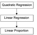
The available data in some server definitions may not be enough for the full Multi-Variable Quadratic Regression. This commonly happens when the server definition only includes 2~3 server configurations. In that case, the interpolation method will degrade, as shown in the following figure.
Figure 494: Secondary Interpolation Method
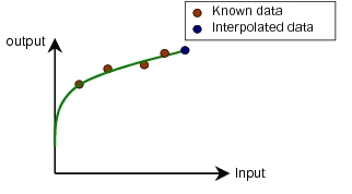
The major difference between the interpolation methods is the method of data regression. The Quadratic Regression tries to find a best fit line using a quadratic function. The following figure shows a Quadratic Regression example in which the input is a single variable.
Figure 495: Quadratic Regression
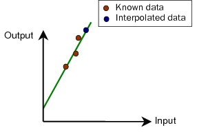
The Linear Regression method tries to find a best fit line using a linear function. The following figure is a Linear Regression example when the input is a single variable.
Figure 496: Linear Regression
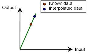
The Linear Proportion is the simplest method. It scales the input data in a linear way. Only one input data point is allowed, and no regression is involved.
Figure 497: Linear Proportion
When not enough data is available to do full Quadratic Regression, the Linear Regression is applied. When the Linear Regression is also not applicable, the Linear Proportion is applied. Since the Linear Proportion only requires one data point, it is applicable for all scenarios.
Server Scaler
The Server Scaler dialog box is accessed from the Protocols > Servers > Upgrade/Downgrade Servers menu. This dialog box lets you rapidly deploy server definitions to one or more servers in the network model. You can select multiple server definitions to deploy and use the << button to make batch changes, or you can drag-and-drop individual server definitions onto individual network objects.
Figure 498: Server Scaler Dialog Box
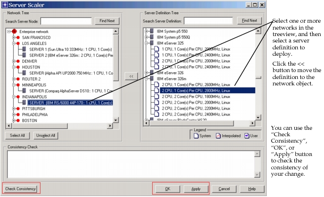
The Check Consistency button executes a check to see if the following two conditions are satisfied:
- The deployed server configuration is located in the external server definition file
- For all server jobs defined on a server node, the corresponding deployed server configuration supports the currently specified job class
Server Simulation Operations
The Server Simulation Operations menu operation (Protocols > Servers > Show/Hide Server Planning Toolbar) brings up a set of selections related to discrete event simulations. From this menu, you can run a simulation, view the results of a simulation, open the Workload Scaler, or calibrate servers automatically.
Figure 499: Server Simulation Operations
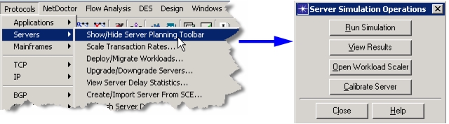
When you select the Calibrate Server button, you can automatically calibrate the I/O subsystem of a server. First you must import data into SCE, classify your processes into jobs, and define a server workload. After calibration, DES results for the workload closely match the actual performance data collected from the server, based on the setting of the Calibration Threshold. See Procedure 107 for more details.
Some important items to remember prior to running calibration are as follows:
- Auto-calibration only works on detailed servers, not simple servers.
Note: To check the server type, right-click on the node in the project editor and select Edit Attributes. Expand the Servers compound attribute, and check the value of Server Modeling Method.
- Set the attribute Servers > Advanced Server Configuration > Storage Partitions > Partition Type to “Local” on servers you want to calibrate. Also ensure that the Measured Access attribute in this table contains appropriate values. The Measured Access attribute is the number the calibration engine will try to match.The values may be filled in based on current information, but you can adjust the values as needed.
- Make sure that the value in Servers > Advanced Server Configuration > Local Storage Subsystem > Interface Configuration > Interface Channels > Disk Configuration > Disk Type matches your actual disk as closely as possible.
Procedure 107: Auto-Calibrate Servers
-
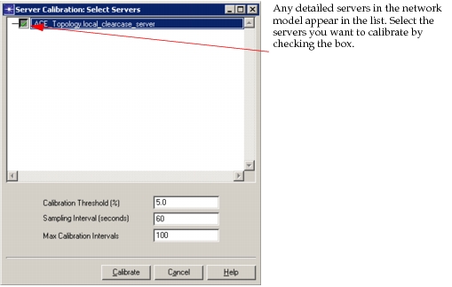
Select Calibrate Server from the Server Simulation Operations dialog box.
Result: The Server Calibration: Select Servers dialog box appears.
Figure 500: Select Servers
-
Select the server(s) you want to calibrate.
-
(Optional) You can set optional parameters for the calibration, or you can choose to accept the default values.
3.1 Set the acceptable Calibration Threshold level in the response time. This value is the percent error that will be tolerated between the measured I/O response and the I/O response determined by DES. For example, a data collector reports an average response time of 5ms for the storage partition C and the calibration threshold is 5%. When calibrating starts, calibration will finish once the DES value is within a +/- 5% of 5ms. This can reduce the amount of time a calibration run takes.
Note: For best results, do not set Calibration Threshold to a value below 2 percent.
3.2 Set the Sampling Interval (Seconds) to the number of seconds between samples. This field specifies the polling interval used by the calibration algorithm. For an I/O intensive server a polling interval of 10 seconds is sufficient, but if the server is relatively idle, you need a longer polling interval. This interval is meant to allow the storage partition average to converge to a stable average.
3.3 Set the Max Calibration Intervals to the number of total calibrations you want to run. This field specifies the maximum number of iterations to try before declaring that a calibration has failed. This value multiplied by the Sampling interval is equal to the maximum simulation time taken in DES.
-
Click the Calibrate button.
Result: A calibration DES is run, and at the end the server will be calibrated
End of Procedure 107
Refresh Server Data
With the menu option Protocols > Servers > Refresh Server Data..., you can deploy system performance data to existing servers in the Project Editor without using SCE. To use this shortcut, you must provide the performance data and an SCE job template to filter the processes into server jobs.
Figure 501: Refresh Server Data
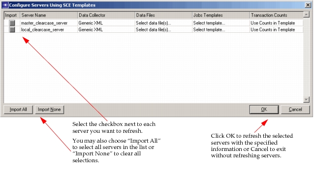
When you select Refresh Server Data..., the dialog box shown in Figure 501 appears. Complete the fields as appropriate for your project. The fields are described below:
- Data Collector—Specifies the type of collector used. Choices are BMC Patrol, HP OVPA - from file, HP OVPA - Connect to OVPM, NetIQ AppManager, Windows Perfmon, or Generic XML.
- Data Files—Specifies the data file containing the performance data. Clicking on this field opens a file chooser window.
- Jobs Template—Specifies the template used to aggregate the process level data into server jobs. Choices are Apache_Server, IIS_Server, Informix_Server, MySQL_Server, Oracle_Server, Sybase_Server, or System.
- Transaction Counts—Specifies the number of transactions in the performance data based on the counts in the template. You can also choose to time-normalize the data.