Creating a New Modulation Curve
A modulation curve characterizes the dependence of the bit error rate (BER) of a radio transmission on the effective signal-to-noise ratio (Eb/No). In network simulations, modulation curves are typically represented by a modulation table (a list of Eb/No - BER values that approximates a continuous modulation curve).
Because the Modulation Curve Editor uses a graphical approach for defining a modulation curve, the resulting data is, inevitably, somewhat imprecise. The most precise way to specify the modulation curve is through EMA code. Modulation curves created via EMA code can still be viewed graphically in the Modulation Curve Editor. For more information on EMA, see “External Model Access” on page 1 in the Model File Access API Reference Manual.
Note: The BER axis of the modulation curve graph is linear, not logarithmic.
Procedure 29: Creating a Modulation Curve
-
In Riverbed Modeler, choose File > New… and select Modulation Curve from the pull-down menu. Click OK.
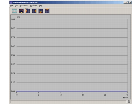
The Modulation Curve Editor opens.
Figure 70: Modulation Curve Editor
-
Use the “Editing a Line Graph” on page 248 operation to specify the line graph.
-
Modify the graph with any of the following operations (all explained in this chapter):
-
Use the Set Abscissa Lower Bound, Set Abscissa Upper Bound, Set Ordinate Lower Bound, and Set Abscissa Upper Bound operations (see Setting Abscissa and Ordinate Bounds) to set the upper and lower values for the gain to any positive or negative integer values. By default, the empty line graph first displayed is set to have a domain of Eb/No values from -10 to 40 and a range of BERs from 0 to 1.0.
Note that upper and lower bounds for the ordinate—the bit error rate—must be between zero and one (0 and 1) inclusive. Also note that upper and lower bounds can be set either before or after a modulation curve is defined. If the bounds are set after a modulation curve is defined, the modulation curve is not changed, but redraws the line graph to match the new range of the ordinate and the new domain of the abscissa.
-
Use the Setting the Sampling Resolution operation to set the number of discrete points along the horizontal axis of the curve. The sampling resolution can be set either before or after a modulation curve is defined. The default sample count is 500.
-
Use the Smoothing a Modulation Curve operation to round out sharp edges in the modulation curve.
-