Analyzing OSPF Networks
Visualizing OSPF Configuration in the Workspace
OSPFv2
You can see which routing protocols are configured on IPv4 physical interfaces by using the View > Visualize Protocol Configuration > IP Routing Protocols > IPv4 Routing Protocols menu operation. This feature adds icons in the Project Editor workspace that indicate which routing protocols are configured in the IPv4 network.
You can also visualize the OSPF areas configured in the network by using the View > Visualize Protocol Configuration > OSPF Area Configuration menu operation. This feature colors the links in the Project Editor workspace according to the OSPF areas. You can specify the color used to represent each area.
OSPFv3
You can see which routing protocols are configured on IPv6 physical interfaces by using the View > Visualize Protocol Configuration > IP Routing Protocols > IPv6 Routing Protocols menu operation. This feature adds icons in the Project Editor workspace that indicate which routing protocols are configured in the IPv6 network.
Viewing the OSPF Routing Table
You can export the OSPF Routing Table on a per-router basis at different times during the simulation. This feature is enabled via the Reports > OSPF Routing Table attribute. The resulting report is available on the Discrete Event Tables tab of the View Results dialog box.
Viewing the OSPF Link State Database
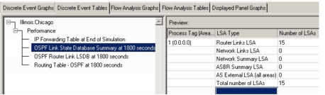
You can export the OSPF Link State Database on a per-router basis at different times during the simulation. This feature is enabled via the Reports > OSPF Link State Database Export attribute. The resulting report is available on the Discrete Event Tables tab of the View Results dialog box.
Figure 423: Results of a Link State Database Export
Available Statistics: OSPF
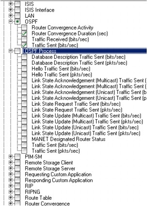
Statistics can be collected during a simulation to analyze OSPF protocol performance. You can analyze the OSPF traffic sent and received at each OSPF enabled router, or all of the OSPF traffic sent across the network. Statistics on the global level and node level are shown in the next two figures.
Figure 424: OSPF Global Statistics
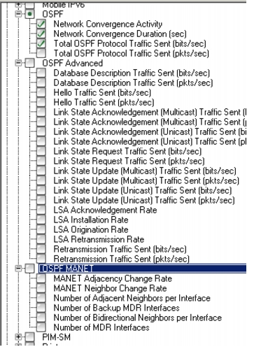
Figure 425: OSPF Node Statistics
Analysis of a Model Using MANET Extensions
You can analyze your OSPFv3 network model that is using MANET extensions by performing the following:
- Mobility analysis
- Results analysis
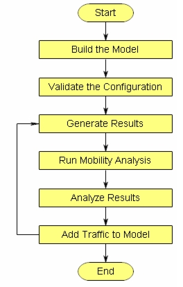
The recommended workflow for building and analyzing your network is shown in the following figure and is described in Procedure 100.
Figure 426: Analyzing the OSPFv3 with MANET Extensions Model
Procedure 100: Analyzing a Model with MANET Extensions
-
Build the model.
1.1 Build your network model with MANET nodes manually, adding a single node at a tine from the object palette, or by using Rapid Configuration. For assistance with building the model, see “Importing and Modeling Networks”
1.2 Add a Mobility Config node from the utilities object palette. Configure profiles to match the behavior you want to model, that is, the speed of the movement of the nodes in the model.
1.3 Add an RX Group Config node from the utilities object palette. Configure this utility node to specify the scope of the graph. This node can limit the transmission range of a mobile node, therefore introducing denseness or sparseness into the network model.
-
Validate the configuration.
Be sure that you follow the guidelines for using MANET extensions in your network model, as described previously in this chapter, and of OSPF networks in general. For instance, all MANET interfaces on the same node must have different BSS IDs regardless of what areas they have. You may also validate your entire network model by using the methods described in the workflow “Validating Imported Network Models”.
-
Generate DES results.
3.1 Select global statistics for OSPF MANET. Global statistics of particular interest when studying mobility are the following:
- Average Number of Adjacencies
- Average Adjacencies Formed
- Average Adjacencies Destroyed
- Average Neighbor Life
- Average Neighbor Change Rate

These statistics are maintained per area and let you see how dynamic the network model is. In particular, the higher the Average Neighbor Life, the less dynamic the network and vice versa.

Average number of adjacencies is useful to determine OSPF scalability in the model. OSPF adjacencies increase linearly with exponentially increasing MANET networks, making OSPF scaleable in MANET environments.

Average Adjacencies Formed and Average Adjacencies Destroyed show how the dynamicity of the MANET network affects OSPF. The higher these rates, the more dynamic the network. Very high adjacency formation and destruction rates introduce instabilities, because nodes are constantly trying to get in sync with each other. In such cases, you can expect a greater number of packet drops, particularly due to routing loops. These rates are function of both the mobility and density of the network. A dense and low mobility network is more stable, whereas a sparse and extremely mobile network is less stable.
3.2 Select OSPF Advanced global statistics. Statistics of particular interest are the following:
- Average Number of Originated LSA
- Average Number of Installed LSA

In a stable network, the average number of installed LSA is roughly equal to the average number of originated LSA times the number of routers in that OSPF area. Since OSPF attempts to ensure that LSAs have been received, an LSA is either retransmitted or, in the case of mobile networks, the next LSA supersedes the previous one.
3.3 Run a DES to assess mobility.
-
Analyze the results.
In global statistics, you can see the total impact of OSPF traffic aggregated across all areas. Examine the number of LSAs originated and installed to determine if there is any instability in the network. Examine the mobility and dynamic nature of the model by analyzing your neighbor statistics.
-
(Optional) Add traffic to the model. If you want to add traffic to the model, use explicit traffic demands. If you need assistance with this step, see “Modeling Additional Traffic”.
Note: Background traffic is not supported on wireless LAN interfaces.
-
(Optional) Run additional analyses. If you make changes to your network model, such as adding traffic, repeat steps 2 through 4.
End of Procedure 100