Understanding and Configuring Statistics Collection
The purpose of this workflow is to describe methods for understanding the way in which statistics are configured and collected for discrete event simulation. The manner in which you configure the collection mode has a direct impact on the resulting statistics and graphs.
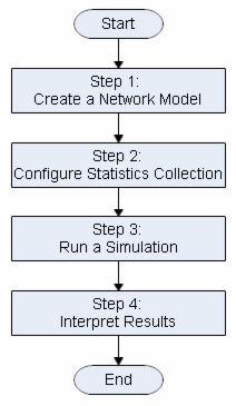
The following figure shows a graphical representation of the workflow described in this document.
Figure 1: Statistics Collection Workflow
Software Components: Understanding/Configuring Statistics Collection
This workflow uses Riverbed analysis software and discrete event simulation (DES).
Prerequisites: Understanding/Configuring Statistics Collection
This workflow requires experience with importing network topologies from available network sources, such as device configuration files or NetCollector.
Workflow Steps: Understanding/Configuring Statistics Collection
The primary steps to configuring statistics collection include
- Step 1: Create a Network Model
- Step 2: Configure Statistics Collection
- Step 3: Run a Simulation
- Step 4: Interpret Results
Step 1: Create a Network Model
Before running simulations, you must create a baseline network model in Riverbed Modeler, as described in the following procedure.
Procedure 1: Creating a Network Model
- Create the network topology.
- Option 1: Create your model manually or by using Rapid Configuration, which will suffice for this workflow.
- Option 2: Model the network topology by importing from device configurations or NetCollector. Be sure to include routing table information, if you want to analyze and validate routing behavior.
- (Optional) Model the network traffic by importing flows, importing link loads, or by configuring manually.
Step 2: Configure Statistics Collection
In selecting the statistics on which you want to report, you may also select the way the data is sampled. By specifying the capture mode and frequency with which data are collected for a statistic, you can reduce the amount of data collected during a simulation. This can significantly reduce the size of the output files and conserve disk space.
The available capture modes are
- All values—collects every data point from a statistic. This mode consumes the most disk space because each data point is logged. The granularity it provides may be beneficial for short studies of a single statistic, however.
- Sample—collects the data according to a user-specified time interval or sample count. For example, if the time interval is 10, data is sampled and recorded once every 10 seconds. If the sample count is 10, every 10th data point is recorded. All other data points are discarded.
- Bucket—collects all of the points over the time interval or sample count into a “data bucket” and generates a result from each bucket.
Procedure 2: Setting the Sample Frequency of a Statistic
-
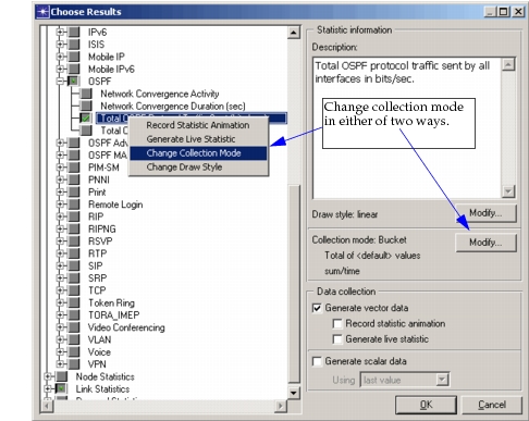
Right-click a statistic name, and choose Change Collection Mode from the Statistic pop-up menu.
Result: A dialog box opens with basic statistic collection options.
Note: If you right-click in the Project Editor and select Choose Individual DES Statistics, you set the collection mode for all objects in the network model. If you right-click on a network object and select Choose Individual DES Statistics, you set the collection mode for only the selected object.
Figure 2: Choose Individual Statistics
-
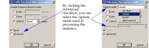
Select the Advanced checkbox.
Result: Pull-down menus for Capture Mode and Bucket Mode are added to the dialog box.
-
Choose the desired capture mode from the Capture Mode pull-down menu: all values, sample, bucket (the default), or glitch removal.
-
Select a radio button for one of the sample frequency modes and enter a frequency value.
Figure 3: Change Collection Mode
Sample-frequency options have different meanings for bucket mode (the default) or sample mode.
The options for bucket mode are:
- Every n seconds—each bucket collects all values generated during n seconds of simulation time. If n equals 10, Riverbed Modeler generates a new value to the output vector after every 10 seconds of simulation time (regardless of how many values are in the bucket). The total number of buckets varies by total simulation time.
- Every n values—collects n values in each bucket. If n equals 10, Riverbed Modeler generates a new value to the output vector whenever a bucket contains 10 values (regardless of how much simulation time has elapsed). The total number of buckets varies by the total number of values.
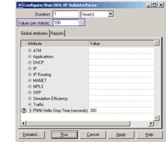
- Total of n values—This is the default mode. The total number of buckets is fixed at n. As in “seconds” bucket mode, each bucket is defined by time: given a simulation duration time of t seconds, and a sample-frequency rate of n, each bucket is the set of all values collected during t/n seconds of simulation time. The number of values in each bucket is not fixed. The default value of n is set by the “Values per Statistic” attribute in the Configure/Run DES Dialog Box, as shown in the following figure. You can change the number of values by changing this number.
Figure 4: Configure/Run Discrete Event Simulation
The options for sample mode are:
- Every n seconds—collects the statistic value at the specified time interval. If n equals 10, data is sampled and recorded once every 10 seconds of simulation time. All other data points are discarded.
- Every n values—collects the statistic value at the specified sample count. If n equals 10, every tenth data point is recorded. All other data points are discarded.
- Total of n values—collects all data up to the specified number of values, either the default set for the statistic (usually 100) or a user-specified number of values. The default value of n is set by the “Values per Statistic” attribute in the Configure/Run DES dialog box.
- 4.1 If using bucket mode, you can also specify how Riverbed Modeler generates a result from each bucket of data. The options on the Bucket mode pull-down menu are:
- max value—The maximum of all the values collected for that bucket period.
- min value—The minimum of all the values collected for that bucket period.
- sum—The sum of all the values collected for that bucket period.
- count—The total number of values collected for that bucket period.
- sample mean—The average of all the values collected for that bucket period.
- time average—The average value where the values that are averaged are weighted according to their duration (where duration is the time between the current value and the next value).
- sum / time—The sum of all the values of points within a particular bucket, divided by the time duration of the bucket.
- summary—The sample mean, the minimum/maximum values, and the standard deviation. Each of these values is graphed separately.
-
(Optional) Set the Reset checkbox. In a few special cases you may want to turn off the Reset checkbox when using bucket mode. With Reset checked (the default position), Riverbed Modeler resets the bucket value to zero after it generates a value and writes it to the output vector. This ensures that each bucket value reflects only the data collected for that bucket. Unchecking Reset causes the bucket value to be retained (not reset to zero) and incorporated into the next bucket. This setting can greatly affect how values are calculated: for example, it determines if the “max value” mode generates the highest value in each bucket (Reset checked) or the highest value generated up to that point (Reset unchecked).
-
Click OK to close the dialog box.
Step 3: Run a Simulation
Now that you have configured the statistics you want to collect and mode in which you want to collect them, run the simulation.
Procedure 3: Running a Simulation
-
Select DES > Configure/Run Discrete Event Simulation.
-
Optionally, click on the Detailed… button to change to the detailed view.
-
Optionally, access promoted attributes by clicking on Object Attributes in the treeview.
Figure 5: Access Promoted Attributes (Detailed View)
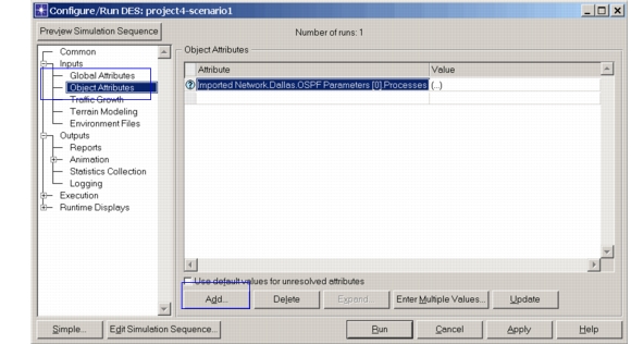
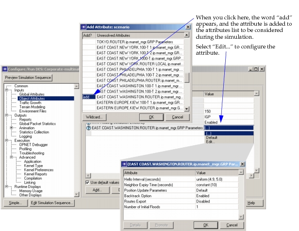
If the attribute you want to modify is not visible, click the Add button and add the attribute and values.
Figure 6: Attribute Parameters
-
Optionally, if you are troubleshooting, enable the debugger.
-
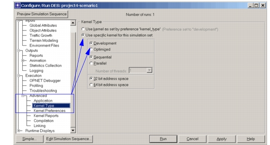
4.1 Select Advanced > Kernel Type, and set the kernel type to Development.
Figure 7: Set Kernel Type to Development (Detailed View)
-
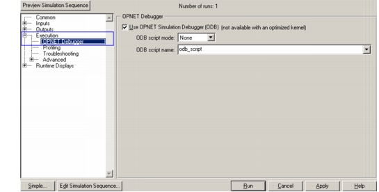
4.2 Select Execution > OPNET Debugger, as shown.
Figure 8: Enable OPNET Debugger (Detailed View)
-
-
Modify any values appropriately. Click the Run button when you are ready to execute the simulation.
-
When the simulation completes, right-click in the project workspace, and select “View Results” to see the DES results for the study.
Step 4: Interpret Results
When you understand how collection is configured, it becomes easier to understand the results you get from a discrete event simulation run. In the following figure, you can see the results for statistic “point-to-point. throughput (bits/sec)” on the link between Paris and Berlin.
Figure 9: View Results of Simulation
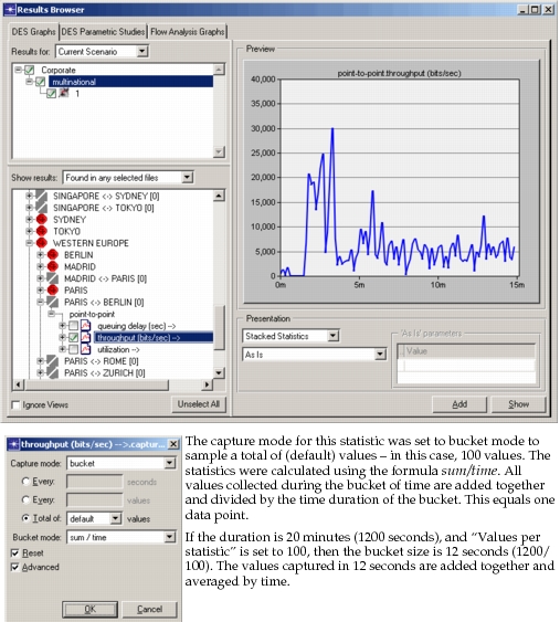
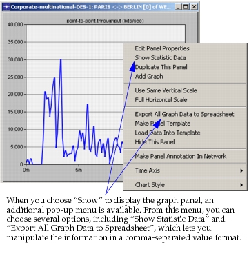
This capture contains samples gathered over a twenty minute period. If you click the “Show” button (see Figure 9), the panel displays individually, as shown in the following figure. As you can see, each data point is displayed in the graph, showing the variation during the simulation.
Figure 10: Graph Panel for Statistic
Graph Results
One point which can be confusing is when you have bursty traffic, yet you never see the peaks of the bursts represented in the graphs. This is because of the way statistics are collected and processed. Consider the following:
- Simulation duration = 1 hour (3600 sim seconds)
- Values per statistic = 100
- Capture mode = bucket mode
- Bucket mode = sum/time
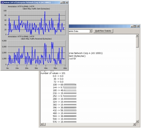
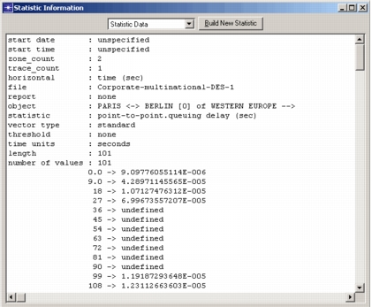
Each bucket is 36 seconds in duration. All values read during the 36-second interval are added together and divided by 36. There are 100 data points resulting. If you right click on a graph panel and choose “Show Statistic Data”, you can view the results as shown in the following figure. For instance, the bucket output at 108 seconds (for a 36-second period) was 0.194444444444. There may have been peaks that were higher than the resulting value, but averaging smoothed the results.
Figure 11: Statistic Data
If we use the sample capture mode with intervals of every 10 seconds, we gather more information (360 data points) without averaging. Although you lose the benefit of longer, averaged samples, you can control the number and type of data points you get.
Figure 12: Sample Mode/10-Second Intervals