Using EMA
Previous topics have introduced the EMA library functions and the Riverbed analysis software models, objects, attributes, and constants. This section presents the details of using EMA for model construction.
Model Construction
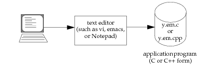
The following figure shows the typical sequence of operations involved in creating models with EMA. The file suffixes identify the different forms of the EMA application. The typical sequence is:
-
Write an application program in C or C++, invoking the correct EMA functions to create and write out an Riverbed model. The file suffix of the application must be
.em.cor.em.cpp, regardless of the model types read or written by the application so that the EMA compilation utilityop_mkemawill recognize the file as an EMA-based application. In this example, the application program is namedy.Figure 11: Creating an EMA Application
-
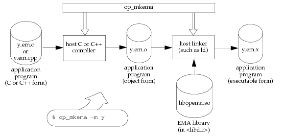
Compile the application program and bind it with the EMA library, using the
op_mkemautility. This utility invokes a compiler defined by the comp_prog or comp_prog_cpp environment attribute (for C or C++, respectively), thereby generating an object code form of the application (with a.em.osuffix). The content of comp_flags or comp_flags_cpp is provided to the compiler. Next,op_mkemainvokes the linker defined by the bind_static_prog environment attribute to combine the application object code and the EMA library into a final executable form (with a.em.xsuffix). A full list ofop_mkemaoptions appears in “op_mkema“ on page 178.Note: To use programs created by
op_mkemaon Linux platforms, you must set the LD_LIBRARY_PATH environment variable manually. For information on setting the LD_LIBRARY_PATH environment variable, see “Linux Installation Troubleshooting“ on page 3.Figure 12: Compiling an EMA Application
-
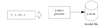
Run the executable form of the application program to create and write out one or more models, which can then be viewed using Riverbed analysis software. In this example, a network model is created.
Figure 13: Executing an EMA Application
The shell command sequence in the following figure replays the preceding scenario for preparation of the y program and the model it produces. The y program generates an indication of the model it produced in this scenario; however, this is not automatically generated by the EMA library.
Figure 14: Compilation of the EMA Application “y”
% vi y.em.c
% op_mkema -m y
--- op_mkema issued the following command: ---
	/bin/sh -c cc -c \
	/usr/riverbed/op_models/y.em.c \
		-I/usr/riverbed/sys/include \
		-o /usr/riverbed/op_models/y.em.o \
	> /usr/riverbed/op_admin/tmp/cc_err 2>&1
--- op_mkema issued the following command: ---
	     /bin/sh -c cc \
	       -o /usr/riverbed/op_models/y.em.x \
	          /usr/riverbed/op_models/y.em.o \
	          -L/usr/riverbed/sys/pc_intel_linux/lib \
	          -lema -lsup -lvos -lmdutl -lmdtab -lmdhndl -lobj -lorb -lprg
	          -lsocket -lm -lc /usr/ucblib/libucb.a \
	        > /usr/riverbed/op_admin/tmp/bind_err 2>&1
-----------------------------------------------
Ema executable program (y.em.x) produced.
-----------------------------------------------
% y.em.x